Empirical Economics
Lecture 1: The Linear Model I
Course Set-Up
Introduction
Empirical Economics
Two central aspects:
- Econometrics and Econometric Theory
- Empirical Practice in the form of programming
Central course objective: to make you understand enough econometric theory, and have you obtain enough experience to :
- Write a succesful thesis (in particular)
- Conduct an empirical economics research project (in general)
Course Layout and Schedule
- Simple course organization: 8 Lectures and 8 Tutorials
- Always: 1 lecture (focused on theory) followed by 1 tutorial (recap and practice)
- Tutorials: Wednesday and Thursday, 13:15-15:15-17:15 (see mytimetable)
- One mid-term (7 Oct) and one end-term exam (7 Nov)
- Organized on Remindo.
- Featuring both multiple choice and open questions akin to the tutorials
Info for students with a disability
You can submit a request for examination accommodations such as exam time extension via OSIRIS Student tab Cases.
Do this by Friday September 12 at the latest. We can then arrange everything before your first exams.
Do you already have provisions from the UU? Then you do not need to submit a request via OSIRIS.
- More information can be found at www.uu.nl/disability
- Questions: students.uu.nl/studyadvisoruse
Lecture Schedule
- Everything is in your timetable, but..
- Lectures: On Friday
- One Exception: No Lecture on Friday 17 October
- Instead: Tuesday 11 October 11:00
- Lectures start at:
- 13:15 (12 Sept, 19 Sept, 3 Oct, 24 October)
- 15:15 (5 Sept, 26 Sept, 10 October)
- Two Q&A Sessions Before Mid-term and End-term Exams:
- Friday 3 October 15:00 (following lecture)
- Friday 24 October 15:00 (following lecture)
Outline
Course Overview
- Linear Model I
- Linear Model II
- Time Series and Prediction
- Panel Data I
- Panel Data II
- Binary Outcome Data
- Potential Outcomes and Difference-in-differences
- Instrumental Variables
What do we do today?
First two lectures devoted to the linear model.
Prequisite knowledge:
- How do we model the processes that might have generated our data?
- How do we summarize and describe data, and try to uncover what process may have generated it?
- Probability and statistics
This lecture and remaining lectures:
- How do we uncover patterns between variables?
- The linear model and further econometrics
Material: Wooldridge Chapters 1 and 2
Prediction vs. Causation
Prediction vs. Causation
Two Distinct Goals: Prediction and Causation
In econometrics, we build models with two primary objectives in mind:
- Predicting an outcome or understanding the causal relationship between variables.
- It is crucial to distinguish between these goals as they dictate our modeling approach and the interpretation of our results.
Prediction
- Prediction is the world of \(\hat{y}\)
- The primary goal of prediction is to forecast the value of a dependent variable (Y) as accurately as possible based on a set of independent variables (X).
- Our focus is on \(\hat{y}\): This is the predicted value of Y generated by our model.
- We build a model that minimizes the difference between the actual values (Y) and the predicted values (\(\hat{y}\)). This difference is known as the residual.
- We are less concerned with the individual coefficients of the independent variables, as long as the model as a whole produces accurate forecasts.
Example: Prediction
Predicting next quarter’s GDP growth using indicators like inflation, consumer confidence, and employment data. The main goal is the accuracy of the GDP forecast (ŷ), not necessarily the isolated impact of each indicator.
Causation
The goal of causal inference is to determine the specific impact of one variable on another, holding all other relevant factors constant.
Our focus is on \(\hat{\beta}\): This is the estimated coefficient of an independent variable. It quantifies the direction and magnitude of the relationship between an independent variable and the dependent variable.
- We aim to obtain an unbiased estimate of the true underlying relationship (\(\beta\)). The “hat” on β means that it is an estimate derived from our sample data.
- What matters most is whether our coefficient \(\hat{\beta}\) is a “good approximation” of the true \(\beta\). We are deeply concerned about issues like omitted variable bias, as they can lead to incorrect conclusions about the causal effect of a variable.
Example: Causation
Estimating the effect of an additional year of education (\(X\)) on an individual’s wages (\(Y\)). We are interested in the specific value of \(\beta\) for education, which would tell us the expected increase in wages for one more year of schooling, assuming other factors are held constant.
Correlation vs. Causation
- If we are interested in causation, we have to be aware of the difference between correlation and causation.
Example: A Causal Effect
Banerjee and Duflo (2015) examined the causal effect of a comprehensive anti-poverty program.
Can a “big push” program, which provides a combination of a productive asset, training, and support, have a lasting causal impact on the lives of the ultra-poor?
To answer this, the researchers used a Randomized Controlled Trial (RCT) across six countries.
- A large number of villages were randomly selected to either receive the program (the “treatment group”) or not (the “control group”).
- This random assignment helps ensure that, on average, the two groups were similar in all other aspects before the program began.
- Therefore, any significant differences observed between the two groups after the program can be causally attributed to the program itself, rather than other factors.
The study found that, even years after the program ended, the treatment group had significantly higher consumption levels and increased income and assets.
Because of the RCT design, the researchers could confidently conclude that the program caused these improvements.
Correlation
- Correlations can be spurious, illustrating a key principle in economics: correlation does not imply causation.
Example: Correlation without Causation
A significant amount of modern finance research focuses on the relationship between a company’s Environmental, Social, and Governance (ESG) scores and its financial performance.
Studies have documented a positive correlation between high ESG scores and strong financial performance.
Companies that score well on environmental and social metrics also tend to be more profitable.
It does not necessarily mean that high ESG scores cause better financial performance. The relationship could be driven by other factors:
- Reverse Causality: It might be that more profitable and successful firms have the resources to invest in improving their environmental and social impact, which in turn leads to higher ESG scores.
- Confounding Variables: A third factor, such as high-quality management, could be responsible for both high ESG scores and strong financial performance. A well-managed company is likely to be both profitable and attentive to its social and environmental responsibilities.
What is Econometrics?
What is Econometrics?
Econometrics is the use of statistical methods to:
- Estimate economic relationships.
- Test economic theories.
- Evaluate and implement government and business policy.
- Forecast economic variables.
It’s where economic theory meets real-world data.
Theory proposes relationships (e.g., Law of Demand), but econometrics tells us the magnitude and statistical significance of these relationships.
Why study econometrics?
It allows you to quantify the relationships that you learn about in your other economics courses.
- By how much does demand fall if we raise the price by 10%?
- What is the effect of an additional year of education on future wages?
- It helps distinguish between correlation and causation.
- It is an essential tool for empirical research in economics and finance, and a highly valued skill in the job market.
The Nature of Economic Data
- The type of data we have determines the econometric methods we should use.
- Cross-Sectional Data: A snapshot of many different individuals, households, firms, countries, etc., at a single point in time.
- Time Series Data: Observations on a single entity (e.g., a country, a company) collected over multiple time periods.
- Pooled Cross-Sections: A combination of two or more cross-sectional datasets from different time periods. The individuals are different in each period.
- Panel (or Longitudinal) Data: The same cross-sectional units are followed over time.
Examples of Economic Data
Examples of Economic Data
Cross-sectional data: A survey of 500 individuals in 2023, with data on their wage, education, gender, and age.
Time-series data: Data on Dutch GDP, inflation, and unemployment from 1950 to 2023.
Pooled cross-sections: A random survey of households in 1990, and another different random survey of households in 2020.
Panel data: Tracking the wage, education, and city of residence for the same 500 individuals every year from 2010 to 2020.
The Concept of a Model
The Population Regression Function (PRF)
- In econometrics, we are interested in relationships between variables.
- Let’s say we are interested in the relationship between wages (\(y\)) and years of education (\(x\)). Economic theory suggests a positive relationship.
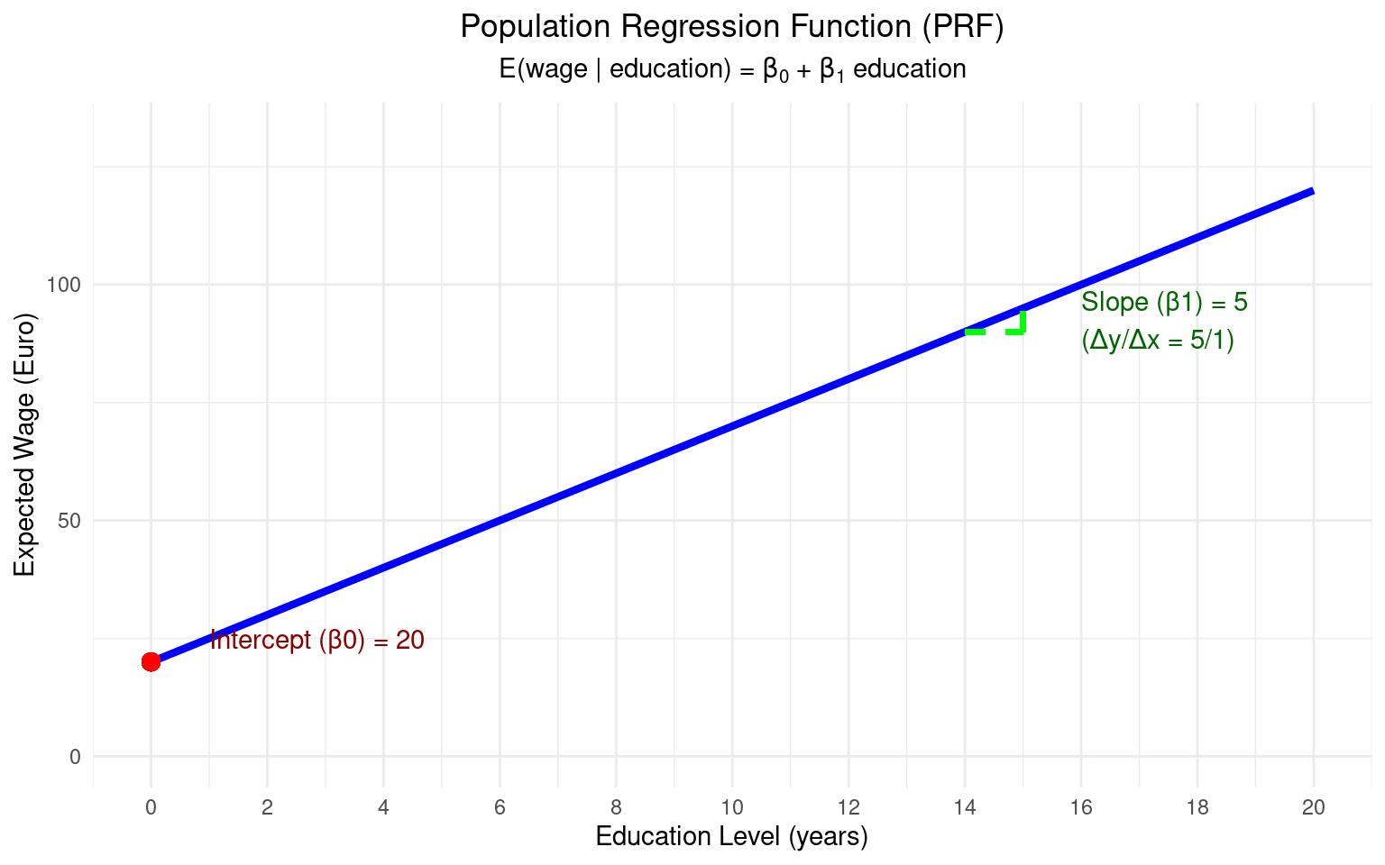
- We can model the average wage for a given level of education. This is the Population Regression Function (PRF):
\[ E(y | x) = \beta_0 + \beta_1 x \]
- Where:
- \(E(y | x)\) is the expected value (average) of y, given a value of x.
- \(\beta_0\) is the population intercept.
- \(\beta_1\) is the population slope. These are unknown constants (parameters) that we want to estimate.
- The PRF represents the true, but unknown, relationship in the population.
Example: Visualization of PRF
The Stochastic Error Term
Of course, not everyone with the same level of education has the same wage. Other factors matter (experience, innate ability, location, luck, etc.).
We capture all these other unobserved factors in a stochastic error term, \(u\).
Our individual-level population model is:
\[ y_i = \beta_0 + \beta_1 x_i + u_i \]
- Where:
- \(y_i\) is the wage of individual \(i\).
- \(x_i\) is the education of individual \(i\).
- \(u_i\) is the error term for individual \(i\). It represents the deviation of individual \(i\)’s actual wage from the population average, \(E(y|x_i)\).
From Population to Sample
We can’t observe the entire population. We only have a sample of data.
Our goal is to use the sample data to estimate the unknown population parameters \(\beta_0\) and \(\beta_1\).
The Sample Regression Function (SRF) is our estimate of the PRF:
\[ \hat{y} = \hat{\beta}_0 + \hat{\beta}_1 x \]
- Where:
- \(\hat{y}\) (y-hat) is the predicted or fitted value of y.
- \(\hat{\beta}_0\) and \(\hat{\beta}_1\) are the estimators of \(\beta_0\) and \(\beta_1\). They are statistics calculated from our sample data.
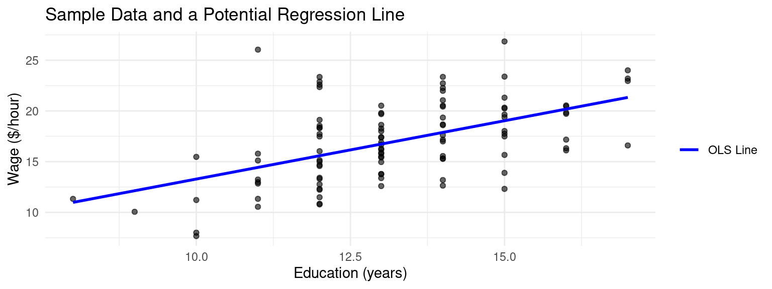
Example Regression in a Sample
Example: Sample Data and Regression
Derivation of the OLS Estimator
Residuals
- How do we choose the “best” values for \(\hat{\beta}_0\) and \(\hat{\beta}_1\)? We want a line that fits the data as closely as possible.
Definition: Residual
We define the residual, \(\hat{u}_i\), as the difference between the actual value \(y_i\) and the fitted value \(\hat{y}_i\): \[ \hat{u}_i = y_i - \hat{y}_i = y_i - (\hat{\beta}_0 + \hat{\beta}_1 x_i) \]
- Note that the residual is different from the error term \(u_i\).
- A residual is the observable difference between the actual data point and the value predicted by your regression model, whereas the unobserved error term \(u_i\) is the theoretical difference between the actual data point and the true, unknown population value.
OLS Method
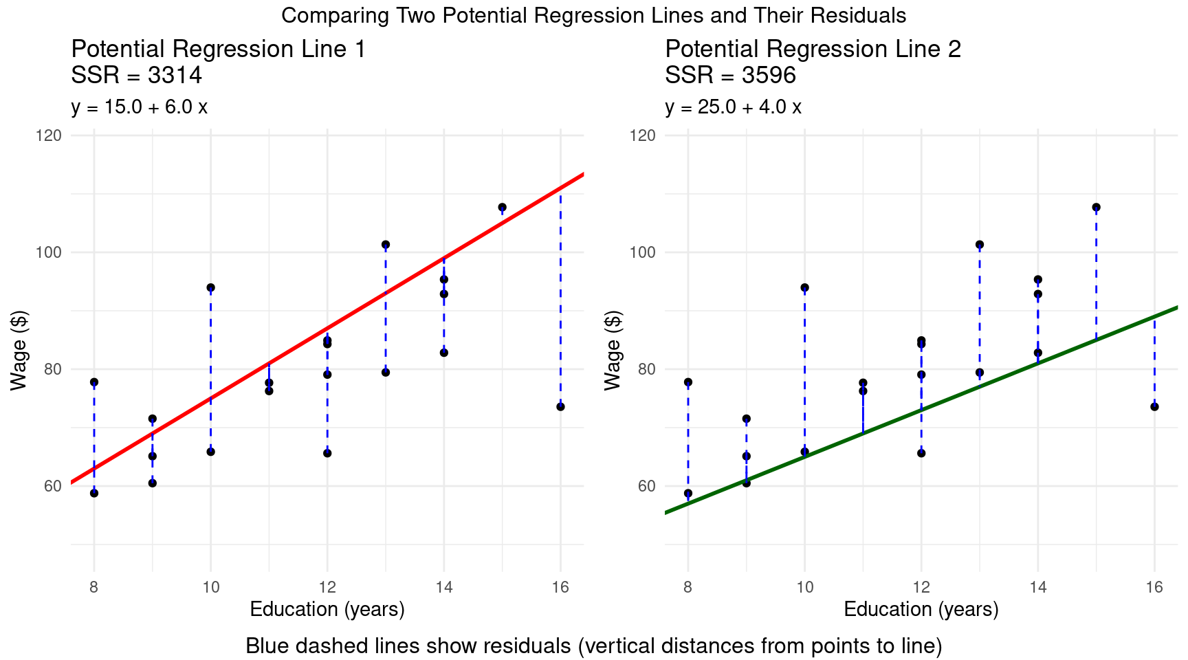
- The Ordinary Least Squares (OLS) method chooses \(\hat{\beta}_0\) and \(\hat{\beta}_1\) to minimize the Sum of Squared Residuals (SSR):
Definition: OLS Optimzation Problem
\[ \min_{\hat{\beta}_0, \hat{\beta}_1} SSR = \sum_{i=1}^{n} \hat{u}_i^2 = \sum_{i=1}^{n} (y_i - \hat{\beta}_0 - \hat{\beta}_1 x_i)^2 \]
- We square the residuals so that positive and negative errors don’t cancel out, and because it penalizes larger errors more heavily.
- This loss function leads to a linear model and it has better statistical properties than other loss functions.
Example: Residuals
Derivation of OLS
- To minimize the SSR, we use calculus: take the partial derivatives with respect to \(\hat{\beta}_0\) and \(\hat{\beta}_1\) and set them to zero.
- These are the First Order Conditions (FOCs).
OLS First Order Conditions
- \(\frac{\partial SSR}{\partial \hat{\beta}_0} = -2 \sum_{i=1}^{n} (y_i - \hat{\beta}_0 - \hat{\beta}_1 x_i) = 0 \implies \sum (y_i - \hat{\beta}_0 - \hat{\beta}_1 x_i) = 0\)
- \(\frac{\partial SSR}{\partial \hat{\beta}_1} = -2 \sum_{i=1}^{n} x_i (y_i - \hat{\beta}_0 - \hat{\beta}_1 x_i) = 0 \implies \sum x_i(y_i - \hat{\beta}_0 - \hat{\beta}_1 x_i) = 0\)
OLS Solution
- Solving this system of two equations for the two unknowns (\(\hat{\beta}_0\), \(\hat{\beta}_1\)) gives the OLS estimator formulas:
Theorem: OLS Estimates for \(\beta_0\) and \(\beta_1\)
\[ \hat{\beta}_1 = \frac{\sum_{i=1}^{n} (x_i - \bar{x})(y_i - \bar{y})}{\sum_{i=1}^{n} (x_i - \bar{x})^2} = \frac{\text{Sample Covariance}(x,y)}{\text{Sample Variance}(x)} \]
\[ \hat{\beta}_0 = \bar{y} - \hat{\beta}_1 \bar{x} \]
where \(\bar{x}\) and \(\bar{y}\) are the sample means of \(x\) and \(y\).
- Note that for \(\beta_1\) to be defined, the Sample Variance in \(x \neq 0\), referred to as no perfect multicollinearity.
Algebraic Properties of OLS
The OLS estimators have some important algebraic properties that come directly from the FOCs:
The sum of the OLS residuals is zero:
- This implies that the sample average of the residuals, \(\bar{u}\), is also zero.
\[\sum_{i=1}^{n} \hat{u}_i = 0\]
Algebraic Properties of OLS (Cont.)
- The sample covariance between the regressor (\(x\)) and the OLS residuals (\(\hat{u}\)) is zero:
- This means the part of \(y\) that we can’t explain with \(x\) (the residual) is uncorrelated with \(x\) in our sample.
\[\sum_{i=1}^{n} x_i \hat{u}_i = 0\]
- The point \((\bar{x}, \bar{y})\) is always on the OLS regression line.
- From the formula \(\hat{\beta}_0 = \bar{y} - \hat{\beta}_1 \bar{x}\), we can write \(\bar{y} = \hat{\beta}_0 + \hat{\beta}_1 \bar{x}\).
Interpreting OLS Coefficients
- Let’s run our wage-education regression: \(\text{Wage}_i = \hat{\beta}_0 + \hat{\beta}_1 \text{Educ}_i\)
Code
slr_model <- lm(wage ~ educ, data = dat)
# The coefficients are:
summary(slr_model)
##
## Call:
## lm(formula = wage ~ educ, data = dat)
##
## Residuals:
##     Min      1Q  Median      3Q     Max
## -6.7201 -2.3878 -0.3926  1.9554 11.6092
##
## Coefficients:
##             Estimate Std. Error t value Pr(>|t|)
## (Intercept)   1.7863     2.5164   0.710    0.479
## educ          1.1498     0.1887   6.092 2.19e-08 ***
## ---
## Signif. codes:  0 '***' 0.001 '**' 0.01 '*' 0.05 '.' 0.1 ' ' 1
##
## Residual standard error: 3.4 on 98 degrees of freedom
## Multiple R-squared:  0.2747, Adjusted R-squared:  0.2673
## F-statistic: 37.11 on 1 and 98 DF,  p-value: 2.192e-08
Code
import statsmodels.api as sm
X = r.dat.educ
y = r.dat.wage
X = sm.add_constant(X)
model = sm.OLS(y, X).fit()
print(model.summary())
##                             OLS Regression Results
## ==============================================================================
## Dep. Variable:                   wage   R-squared:                       0.275
## Model:                            OLS   Adj. R-squared:                  0.267
## Method:                 Least Squares   F-statistic:                     37.11
## Date:                Wed, 29 Oct 2025   Prob (F-statistic):           2.19e-08
## Time:                        12:56:43   Log-Likelihood:                -263.27
## No. Observations:                 100   AIC:                             530.5
## Df Residuals:                      98   BIC:                             535.8
## Df Model:                           1
## Covariance Type:            nonrobust
## ==============================================================================
##                  coef    std err          t      P>|t|      [0.025      0.975]
## ------------------------------------------------------------------------------
## const          1.7863      2.516      0.710      0.479      -3.207       6.780
## educ           1.1498      0.189      6.092      0.000       0.775       1.524
## ==============================================================================
## Omnibus:                        8.366   Durbin-Watson:                   2.235
## Prob(Omnibus):                  0.015   Jarque-Bera (JB):                8.006
## Skew:                           0.626   Prob(JB):                       0.0183
## Kurtosis:                       3.595   Cond. No.                         99.2
## ==============================================================================
##
## Notes:
## [1] Standard Errors assume that the covariance matrix of the errors is correctly specified.- So our estimated SRF is: \(\widehat{Wage} = 1.79 + 1.15 \times Educ\)
Interpretation
- Slope (\(\hat{\beta}_1 \approx 1.15\)): “For each additional year of education, we estimate the hourly wage to increase by €1.15, on average.” This is the key policy parameter.
- Intercept (\(\hat{\beta}_0 \approx 1.79\)): “For an individual with zero years of education, we predict an hourly wage of €1.79.”
Units and Functional Form
The values of the coefficients depend on the units of measurement of \(y\) and \(x\). We’ve used a level-level model (\(y\) and \(x\) are in their natural units).
Suppose we measured wage in cents instead of euros.
- The new dependent variable is \(Wage_{cents} = 100 \times Wage\).
- The new regression would be: \(\widehat{Wage_{cents}} = (100 \times \hat{\beta}_0) + (100 \times \hat{\beta}_1) \times Educ\)
- Both the intercept and slope would be 100 times larger. The interpretation is the same, just the units change (“an extra year of education increases wage by 125 cents”).
Units and Functional Form (Cont.)
- What if we measured education in months instead of years?
- The interpretation of \(\hat{\beta}_1\) would become “the estimated change in wage for an additional month of education.” The coefficient value would be \(\frac{1}{12}\) of its original value:
Example: Education in Months
From our definition, \(Educ_{years} = \frac{1}{12} Educ_{months}\). Let’s substitute this into the original estimated equation:
\[\begin{align*} \widehat{Wage} &= \hat{\beta}_0 + \hat{\beta}_1 Educ_{years} \\ &= \hat{\beta}_0 + \hat{\beta}_1 \left( \frac{1}{12} Educ_{months} \right) \\ &= \hat{\beta}_0 + \left( \frac{\hat{\beta}_1}{12} \right) Educ_{months} \end{align*}\]
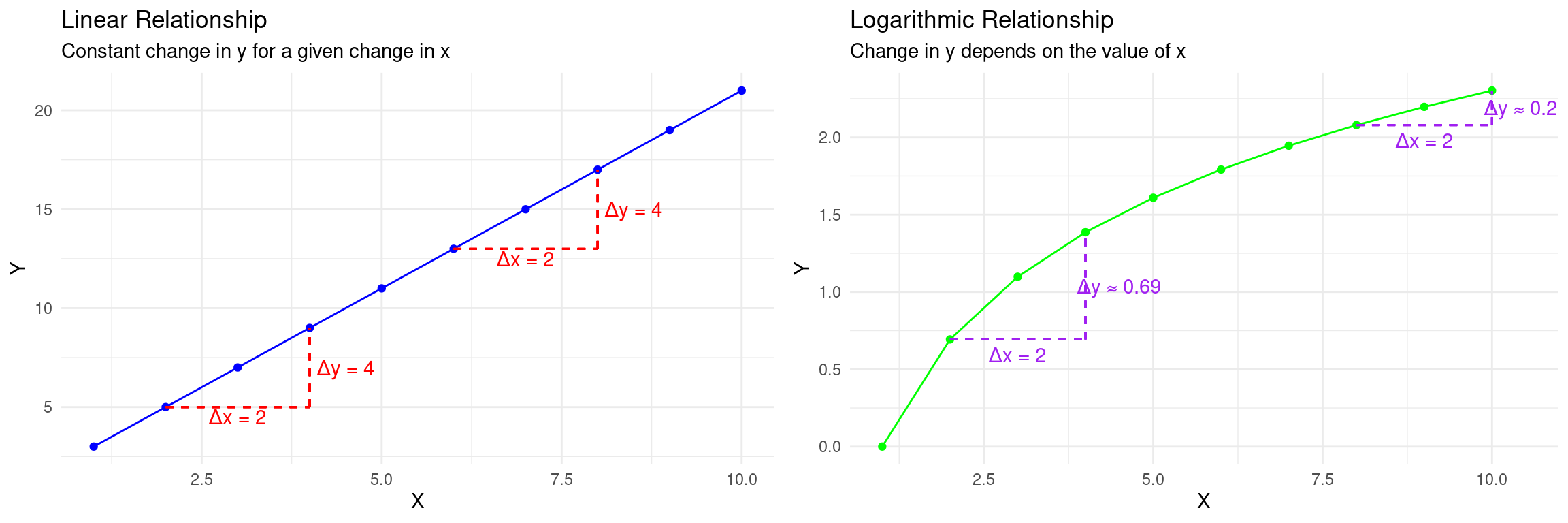
Why use different functional forms?
- So far, we’ve assumed a linear relationship: a one-unit change in \(x\) leads to the same change in \(y\), regardless of the value of \(x\).
- But often, relationships are not linear. We use transformations (like logarithms) to:
- Model Non-Linear Relationships: Capture effects that are proportional or diminishing.
- Change the Interpretation: Analyze percentage changes instead of unit changes.
- Improve Statistical Properties: Stabilize the variance of the error term or make the distribution of a variable more symmetric.
The Log-Level Model: \(\log(y)\) on \(x\)
Here, we transform the dependent variable \(y\): \(\log(y) = \beta_0 + \beta_1 x + u\)
Interpretation of \(\beta_1\): A one-unit increase in \(x\) is associated with a \((100 \times \beta_1)\%\) change in \(y\).
Interpretation of \(\beta\) in the Log-Level Model
To see this, take the derivative of the equation with respect to \(x\): \[ \frac{d(\log(y))}{dx} = \beta_1 \]
Recall the calculus rule/approximation: for small changes, \(\Delta \log(y) \approx \frac{\Delta y}{y}\).
For a one-unit change in \(x\) (\(\Delta x = 1\)): \[ \beta_1 = \frac{\Delta \log(y)}{\Delta x} \approx \frac{\Delta y / y}{1} \]
Example Log-Level
Example: Log-Level Interpretation
In a log-level model, \(\beta_1\) is the proportional change in \(y\).
We multiply by 100 to get a percentage.
If \(\widehat{\log(Wage)} = 1.5 + 0.08 \times Educ\), an additional year of education is associated with an approximate \(0.08 \times 100 = 8\%\) increase in wage.
The Level-Log Model: \(y\) on \(\log(x)\)
Here, we transform the independent variable \(x\): \(y = \beta_0 + \beta_1 \log(x) + u\)
Interpretation of \(\beta_1\): A 1% increase in \(x\) is associated with a \((\beta_1 / 100)\) unit change in \(y\).
Interpretation of \(\beta\) in Level-Log Model
To see this, take the derivative of the equation with respect to \(\log(x)\): \[ \frac{dy}{d(\log(x))} = \beta_1 \]
A change in \(\log(x)\) is approximately the proportional change in \(x\): \(\Delta \log(x) \approx \frac{\Delta x}{x}\).
- So, \(\Delta y \approx \beta_1 \Delta(\log(x)) \approx \beta_1 \frac{\Delta x}{x}\).
- If we consider a 1% change in \(x\), then \(\frac{\Delta x}{x} = 0.01\).
- The resulting change in \(y\) is: \(\Delta y \approx \beta_1 \times (0.01) = \frac{\beta_1}{100}\).
Example Level-Log Model
Example: Level-Log Model
Suppose that the estimated regression model linking advertising expenditure to monthly sales revenue is:
\[ \text{Monthly Sales Revenue} = 50 + 12 \times \log(\text{Monthly Advertising Spending}) \]
In this model, Monthly Sales Revenue (Y) is measured in thousands of euros (Level), and Monthly Advertising Spend (X) is measured in euros (Log).
A 1% increase in Monthly Advertising Spend is associated with a \(12/100 = 0.12\) increase in Monthly Sales Revenue. Since Sales Revenue is measured in thousands of euros, a 1% increase in advertising spend is associated with a €120 increase in monthly sales revenue (\(0.12 \times €1,000 = €120\)).
The Log-Log Model: \(\log(y)\) on \(\log(x)\)
- This model is very common in economics: \(\log(y) = \beta_0 + \beta_1 \log(x) + u\)
Interpretation of \(\beta\) in the Log-Log Model
A 1% increase in \(x\) is associated with a \(\beta_1\%\) change in \(y\). To see this, from the model, we can write: \[ \beta_1 = \frac{d(\log(y))}{d(\log(x))} \]
Using the same approximations as before: \[ \beta_1 \approx \frac{\Delta y / y}{\Delta x / x} = \frac{\%\Delta y}{\%\Delta x} \]
- If we set the percentage change in \(x\) to 1% (\(\%\Delta x=1\)), then the percentage change in \(y\) is just \(\beta_1\).
Example Log-Log Form
Example: Interpretation of \(\beta_1\) in the Log-Log Model
Suppose we have estimated \(\log(\text{Sales}) = 4.8 - 1.2 \times \log(\text{Price})\) for a product. Then, a 1% increase in price is associated with a 1.2% decrease in sales.
Other Forms: Polynomials
- We can also add polynomial terms (like \(x^2\), \(x^3\), etc.) to capture more complex non-linear patterns, such as diminishing returns.
- Model (Quadratic): \(y = \beta_0 + \beta_1 x + \beta_2 x^2 + u\)
- This is another example where if \(x_i\) differs among individuals, different individuals have different marginal effects.
Interpretation of the Quadratic Model
The effect of a change in \(x\) on \(y\) now depends on the level of \(x\).
The marginal effect of \(x\) on \(y\) is the derivative with respect to \(x\): \[ \frac{\Delta y}{\Delta x} \approx \frac{dy}{dx} = \beta_1 + 2 \beta_2 x \]
A one-unit change in \(x\) is associated with a change in \(y\) of approximately \(\beta_1 + 2 \beta_2 x\).
Example Polynomial
Example: Polynomial Regression
Suppose we have estimated a model for annual income based on a worker’s age:
\(\widehat{Income} = 20,000 + 1,500 \times Age - 20 \times Age^2\).
The effect of the first year of work experience (e.g., going from age 20 to 21) is approximately: \(1,500 + 2(-20)(20) = 1,500 - 800 = \$700\).
The effect of gaining one more year of experience when a worker is 40 (i.e., going from age 40 to 41) is: \(1,500 + 2(-20)(40) = 1,500 - 1,600 = -\$100\).
This captures the common life-cycle pattern of earnings: income rises with age and experience, but at a decreasing rate, and may eventually begin to decline after a certain point. This demonstrates the diminishing returns to age and experience on income.
Dummy Variables
- A dummy variable (or indicator variable), \(D_i\), is a special variable: a binary variable that takes the value 1 if an observation \(i\) belongs to a specific category, and 0 otherwise.
- This allows us to incorporate qualitative information (e.g., gender, policy status, geographic region) into a regression model.
Example: Wage Conditional on Gender Dummy
Consider a regression of wage on a single dummy variable for gender:
\[ Wage_i = \beta_0 + \beta_1 Female_i + u_i \]
where \(Female_i = 1\) if person i is female, and \(Female_i = 0\) if male.
Interpretation
- To interpret the coefficients, we take the conditional expectation of
wagefor each group:
Example: Wage on Gender (Cont.)
- For Males (\(Female_i = 0\)):
- \(E[Wage_i | Female_i=0] = \beta_0 + \beta_1(0) = \beta_0\)
- The expected wage for the reference group (males) is simply the intercept, \(\beta_0\).
- For Females (\(Female_i = 1\)):
- \(E[Wage_i | Female_i=1] = \beta_0 + \beta_1(1) = \beta_0 + \beta_1\)
- The expected wage for the treatment group (females) is \(\beta_0 + \beta_1\).
The coefficient \(\beta_1\) represents the difference in the expected outcome between the two groups:
\[ E[Wage_i | Female_i=1] - E[wage_i | Female_i=0] = (\beta_0 + \beta_1) - \beta_0 = \beta_1 \]
Now, \(\beta_1\) is the average difference in wages between females and males.
Summary of Interpretations
| Model Name | Equation | Interpretation of \(\hat{\beta}_1\) |
|---|---|---|
| Level-Level | \(y = \beta_0 + \beta_1 x\) | A 1-unit change in \(x\) leads to a \(\hat{\beta}_1\) unit change in \(y\). |
| Log-Level | \(\log(y) = \beta_0 + \beta_1 x\) | A 1-unit change in \(x\) leads to a \((100 \times \hat{\beta}_1)\%\) change in \(y\).1 |
| Level-Log | \(y = \beta_0 + \beta_1 \log(x)\) | A 1% change in \(x\) leads to a \((\hat{\beta}_1/100)\) unit change in \(y\). |
| Log-Log | \(\log(y) = \beta_0 + \beta_1 \log(x)\) | A 1% change in \(x\) leads to a \(\hat{\beta}_1\%\) change in \(y\). |
| Polynomial | \(y = \beta_0 + \beta_1 x + \beta_2 x^2 + \dots\) | A 1-unit change in \(x\) leads to a \(\hat{\beta}_1 + 2 \hat{\beta}_2 x\) change in \(y\). |
| Dummies | \(y = \beta_0 + \beta_1 D_i\) | Relative to the reference category, the 1 category has a \(\hat{\beta}_1\) lower/higher \(y\). |
Goodness of Fit
Goodness-of-Fit
How well does our estimated line explain the variation in our dependent variable, \(y\)?
We can partition the total variation in \(y\) into two parts: the part explained by the model, and the part that is not explained.
Partition of Variation in \(Y\)
SST (Total Sum of Squares): Total variation in \(y\). \(SST = \sum (y_i - \bar{y})^2\)
SSE (Explained Sum of Squares): Variation explained by the regression. \(SSE = \sum (\hat{y}_i - \bar{y})^2\)
SSR (Sum of Squared Residuals): Unexplained variation. \(SSR = \sum \hat{u}_i^2\)
If the regression equation includes a constant term, it is a mathematical property that SST = SSE + SSR.
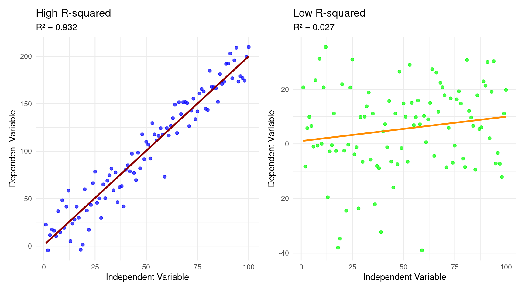
Goodness-of-Fit: \(R^2\)
- We want to encapsulate “goodness-of-fit” into one number.
Definition: \(R^2\)
The R-squared measures the proportion of the total sample variation in \(y\) that is “explained” by the regression model.
\[ R^2 = \frac{SSE}{SST} = 1 - \frac{SSR}{SST} \]
- \(R^2\) is always between 0 and 1.
- A higher \(R^2\) means the model fits the data better in-sample.
- Caution: A high \(R^2\) is not the ultimate goal of econometrics! We care more about getting an unbiased estimate of the causal effect \(\beta_1\).
\(R^2\) Visualization
OLS Classical Assumptions
Unbiasedness
- A key desirable property of an estimator is unbiasedness.
- The objective of a regression is to say something about the population parameters \(\beta\). However, we only have a sample equivalent, \(\hat{\beta}\) at our disposal.
- This estimate goes paired with some uncertainty.
Definition: Unbiasedness
An OLS estimator is considered unbiased if its expected value, across many hypothetical samples, is equal to the true population parameter it is intended to estimate. Mathematically, for a regression coefficient \(\beta\), its OLS estimator \(\hat{\beta}\) is unbiased if:
\[ E[\hat{\beta}] = \beta \]
Unbiasedness Implication
- This does not imply that an estimate from any single sample will be the true population parameter.
- Instead, it means that if we were to draw an infinite number of random samples from the population and compute the OLS estimate for each, the average of these estimates would be equal to the true value of \(\beta\).
- This property ensures that, on average, the OLS procedure does not systematically overestimate or underestimate the true parameter.
The SLR Assumptions
- When does unbiasedness hold?
- For our OLS estimates to have desirable statistical properties, certain assumptions must hold. These are the SLR Assumptions.
SLR Assumptions
- Assumption 1: Linearity in Parameters. The population model is \(y = \beta_0 + \beta_1 x + u\).
- Assumption 2: Random Sampling. The data \((x_i, y_i)\) are a random sample from the population described by the model.
- Assumption 3: Sample Variation in \(x\). The values of \(x_i\) in the sample are not all the same. This is the no perfect collinearity assumption.
- Assumption 4: Zero Conditional Mean. \(E(u|x) = 0\). The average value of the unobserved factors is unrelated to the value of \(x\).
Unbiasedness of OLS
Theorem: Unbiasedness of OLS
Under assumptions SLR.1 through SLR.4, the OLS estimators are unbiased.
\[ E(\hat{\beta}_0) = \beta_0 \quad \text{and} \quad E(\hat{\beta}_1) = \beta_1 \]
- What does this mean?
- Unbiasedness is a property of the OLS estimator given the assumptions.
- If we could draw many, many random samples (with the same \(n\)) from the population and calculate \(\hat{\beta}_1\) for each sample, the average of all these estimates would be equal to the true population parameter, \(\beta_1\).
- Our estimate from any single sample might be higher or lower than the true value, but on average, we get it right.
- This property relies critically on the Zero Conditional Mean assumption (SLR.4). If SLR.4 fails, OLS is biased.
- Unbiasedness is a property of the OLS estimator given the assumptions.
Violation of Unbiasedness
Assumption 4, \(E(u|x) = 0\), is the most important assumption for establishing causality.
- It means that the explanatory variable (\(x\)) must not be correlated with any of the unobserved factors (\(u\)) that affect the dependent variable (\(y\)).
When is unbiasedness violated?
An important reason arises when a relevant explanatory variable is excluded from the model, referred to as Omitted Variable Bias.
- This omission leads to biased and inconsistent estimates for the coefficients of the included variables.
For OVB to exist, two conditions must be met:
- The omitted variable must be a determinant of the dependent variable (i.e., its true coefficient is not zero).
- The omitted variable must be correlated with at least one of the included independent variables.
When these conditions hold, the OLS estimator for the included variable’s coefficient mistakenly incorporates the effect of the omitted variable, leading to a biased result.
- This violates the crucial OLS assumption that the error term is uncorrelated with the regressors.
Prediction of Direction of Bias
- The direction of the bias is determined by the signs of these two key relationships.
Omitted Variable Bias Definition
Consider the true regression model: \(y = \beta_0 + \beta_1 x_1 + \beta_2 x_2 + u\), where \(x_2\) is the omitted variable.
Instead, we estimate the simpler model \(y = \alpha_0 + \alpha_1 x_1 + v\). The bias in the estimate of \(\alpha_1\) can be expressed as:
\[ \text{Bias} = E[\hat{\alpha_1}] - \beta_1 = \beta_2 \cdot \delta_1 \]
Where:
- \(\beta_2\) is the true coefficient of the omitted variable (\(X_2\) in the correctly specified model. This represents the partial effect of \(X_2\) on Y.
- \(\delta_1\) is the coefficient from an auxiliary regression of the omitted variable (\(X_2\)) on the included variable (\(X_1\)): \(X_2 = \delta_0 + \delta_1 X_1 + w\). This represents the correlation between \(X_1\) and \(X_2\).
Examples of OVB
- The direction of the bias can be predicted by the product of the signs of \(\beta_2\) and \(\delta_1\):
Examples: OVB
Suppose we estimate \(\text{Wage} = \beta_0 + \beta_1 \text{Education} + u\), but there is an omitted variable \(X_2\), Innate Ability. The resulting coefficient will be an oversestimate of the true effect:
- Sign of $_2 (Effect of \(X_2\) on \(Y\)): The sign is positive (+). It is widely accepted that, holding education constant, individuals with higher innate ability tend to earn higher wages. This is because ability is a component of a worker’s overall productivity.
- Sign of \(\delta_1\) (Correlation of \(X_2\) with \(X_1\)): The sign is positive (+). Individuals with higher innate ability are often more likely to attain higher levels of education. They may find schooling less challenging and have greater incentives to pursue further education.
- The formula for the bias is \(\text{Bias}=\beta_2 \cdot \delta_1\). Therefore, the predicted direction is
(+) * (+) = +.
Examples of OVB (Cont.)
Examples: OVB
Suppose we estimate the model \(\text{Educational_Outcome} = \beta_0 + \beta_1 \text{Class Size} + u\), with the omitted variable \(X_2\) being a student’s socioeconomic background or level of need. The resulting bias is positive (leading to an underestimation of a negative effect):
- Sign of \(\beta_2\) (Effect of \(X_2\) on \(Y\)): The sign is negative (-). Students from disadvantaged socioeconomic backgrounds or with higher needs tend to have, on average, lower educational outcomes. This can be due to fewer resources at home, less parental support, and other related challenges.
- Sign of \(\delta_1\) (Correlation of \(X_2\) with \(X_1\)): The sign is negative (-). School districts often purposefully create smaller classes for students who require more attention, such as those from lower-income families, or students with learning disabilities. Therefore, a higher prevalence of disadvantaged students is correlated with smaller class sizes.
- Therefore, the predicted direction is
(-) * (-) = +.
Examples OVB (Cont.)
Examples: OVB
Suppose we estimate \(\text{Profits} = \beta_0 + \beta_1\text{Firm Size} + u\), with the omitted variable \(X_2\) being Quality of Management. The resulting bias is positive, resulting in overestimation of the effect.
- Sign of \(\beta_2\) (Effect of \(X_2\) on \(Y\)): The sign is positive (+). High-quality management is a critical factor in a firm’s success and is directly and positively related to higher profitability. Better managers make more effective strategic, operational, and financial decisions.
- Sign of \(\delta_1\) (Correlation of \(X_2\) with \(X_1\)):The sign is positive (+). Larger firms are often able to attract and retain higher-quality managerial talent. They can offer more competitive compensation packages, provide more extensive career opportunities, and may have more sophisticated recruitment processes. Conversely, better management may also lead to firm growth, increasing its size.
- Therefore, the predicted direction is
(+) * (+) = +.
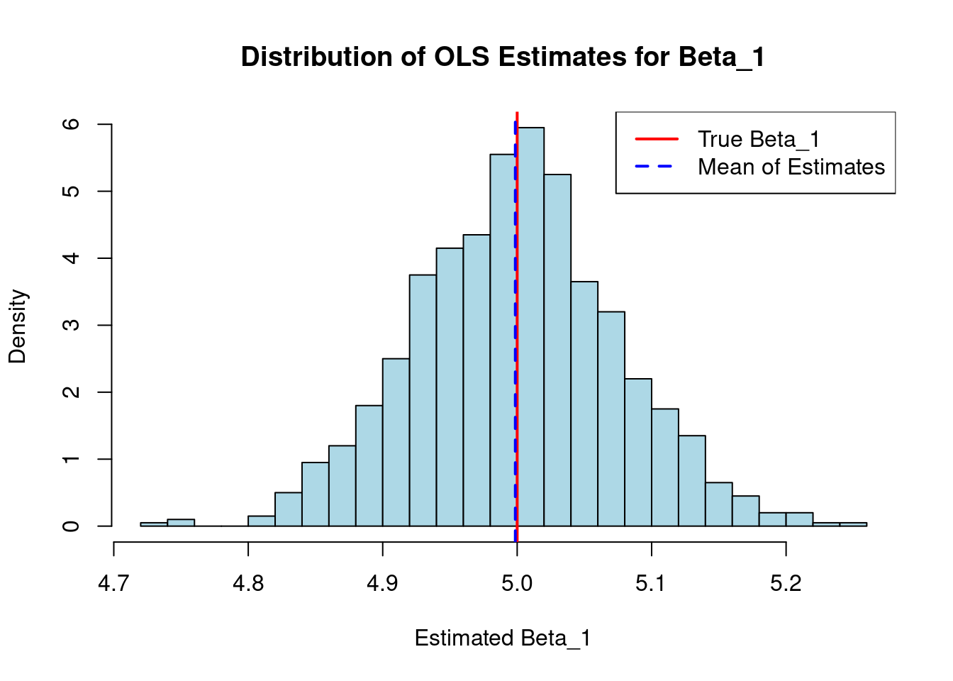
Visualization Unbiasedness
- The true values for the intercept are \(\beta_0=2\) and the slope \(\beta_1=5\) of our hypothetical linear model.
- We then perform an OLS regression 1,000 times.
- In each iteration, it generates a random sample of 100 observations for the variables \(x\) and \(y\) based on the true model, including a random error term.
- For each of these samples, we run a linear regression function and store and plot the estimated coefficient for \(x\):
Variance of OLS Estimators
- We also want our estimators to be precise, meaning they don’t vary too much from sample to sample. This is measured by their sampling variance.
Theorem: Variance of the OLS Estimator
Under assumptions SLR.1 through SLR.5 (all four SLR assumptions plus homoskedasticity), the estimated variance of the OLS slope estimator is:
\[ \widehat{Var}(\hat{\beta}_1) = \frac{\hat{\sigma}^2}{\sum_{i=1}^n (x_i - \bar{x})^2} = \frac{\hat{\sigma}^2}{SST_x} \]
Variance of OLS Estimators (Cont.)
- Let’s forget regression for a second.
- How much does a simple sample mean (\(\bar{x}\)) wobble?
- Its variance (under random sampling) is famously simple: \(Var(\bar{x}) = \frac{\sigma^2}{n}\)
- This formula is driven by two intuitive ideas:
- \(\sigma^2\) is the variance of the underlying population. It’s the inherent “noisiness” or “spread” of the data points themselves.
- \(n\) is your sample size. It’s how much data you have to “anchor” your estimate.
- Looking at \(\widehat{Var}(\hat{\beta}_1) = \frac{\hat{\sigma}^2}{\sum_{i=1}^n (x_i - \bar{x})^2} = \frac{\hat{\sigma}^2}{SST_x}\) tells us the exact same..
Determinants of the Variance
- What determines the precision of our estimate?
- The error variance, \(\sigma^2\): More “noise” in the relationship (larger \(\sigma^2\)) leads to a larger variance for \(\hat{\beta}_1\).
- The total sample variation in \(X\), \(SST_x\): More variation in our explanatory variable (\(x\)) leads to a smaller variance for \(\hat{\beta}_1\). We learn more about the slope when our \(x\) values are more spread out.
- The sample size, \(n\): A larger sample size generally increases \(SST_x\), which decreases the variance of \(\hat{\beta}_1\).
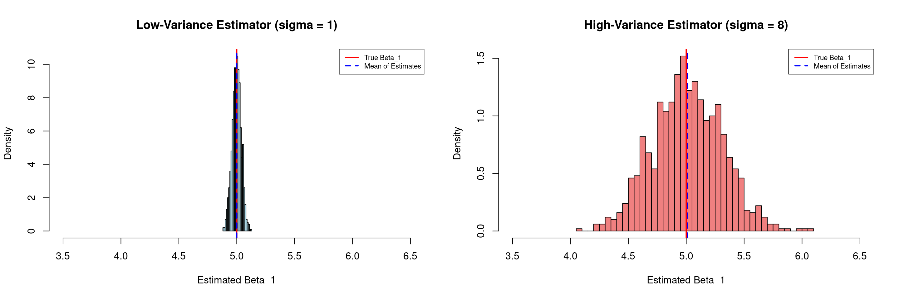
Variance Illustration (Dependence on \(\hat{\sigma}\))
- We plot the distribution of the 1,000 estimated coefficients, which is centered around the true value of 5 (the solid red line).
- In the left panel below, we have a low-variance estimator (\(\sigma=1\))
- The histogram on the right is much narrower and more peaked. The estimates are tightly clustered around the true value.
- In the right panel below, we have a high-variance estimator (\(\sigma=8\))
- The histogram on the right is visibly wider and flatter. This indicates a larger spread in the estimated coefficients. Any single estimate from a sample of this size could be quite far from the true value.
- In the left panel below, we have a low-variance estimator (\(\sigma=1\))
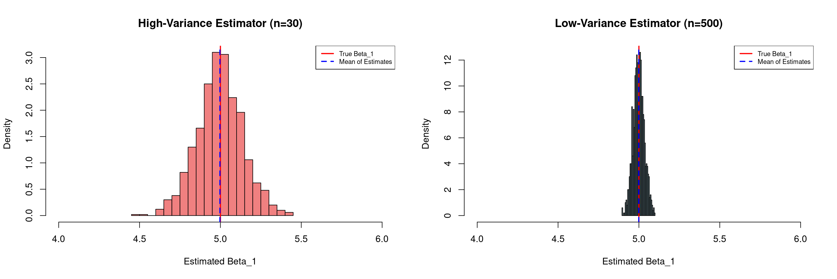
Variance Illustration (Dependence on \(N\))
- We plot the distribution of the 1,000 estimated coefficients, which is centered around the true value of 5 (the solid red line).
- In the left panel below, we have a high-variance estimator (n=30)
- The histogram on the left is visibly wider and flatter. This indicates a larger spread in the estimated coefficients. Any single estimate from a sample of this size could be quite far from the true value.
- In the right panel below, we have a low-variance estimator (n=500)
- The histogram on the right is much narrower and more peaked. The estimates are tightly clustered around the true value.
- In the left panel below, we have a high-variance estimator (n=30)
Variance Illustration (Dependence on \(N\))
- This demonstrates that with a larger sample size, the OLS estimator is more efficient
- We can be more confident that any single estimate is close to the true population parameter
- The mean of the estimates in both scenarios (the dashed blue line) is very close to the true value, confirming that both estimators are unbiased.
Determining the Variance in Practice
- In theory, to know the true variance of the OLS estimator, we need \(\sigma^2\) (the true variance of the errors) for our formula.
- But we can never know the true errors, because we don’t know the true line!
- All we have are the residuals (\(e_i\)) from our estimated line: \(e_i = y_i - \hat{y}_i\)
- Solution: We use the residuals to estimate the error variance. We call this estimate \(s^2\) or \(\hat{\sigma}^2\), and its square root is called the standard error of a regression coefficient.
- On the basis of this estimate, we estimate the sample variance for our estimate \(\hat{\beta}\). Hence our terminology of \(\widehat{Var}(\hat{\beta})\).
The Standard Error
- Our starting point is the computation of the standard error of a regression (SER).
- The SER is an estimator of the standard deviation of the population error term, \(\sigma\). It measures the typical size of a residual (the model’s “average mistake”).
Definition: Standard Error of a Regression
\[ \hat{\sigma} = SER = \sqrt{\frac{SSR}{n-2}} = \sqrt{\frac{\sum e_i^2}{n-2}} \]
- We divide by \(n-2\) (degrees of freedom) because we had to estimate two parameters (\(\beta_0, \beta_1\)) to get the residuals.
- SER is measured in the same units as \(y\). A smaller SER is better.
From Standard Error to Inference
- Now we have all the pieces:
- Start with the true (but unusable) variance formula \(Var(\hat{\beta}_1) = \frac{\sigma^2}{\sum_{i=1}^n (x_i - \bar{x})^2}\)
- Plug in our estimate \(\hat{\sigma}\) for the unknown \(\sigma\) (the SER).
- This gives us the estimated variance: \(\hat{\sigma}^2 / \sum (X_i - \bar{X})^2\)
- Take the square root to get it back to the original units of \(\beta_1\):
- This is the Standard Error of the \(\beta_1\) coefficient.
Definition: Standard Error of a Coefficient
\[ SE(\hat{\beta}) = \hat{\sigma} / \sqrt{\sum_{i=1}^n (X_i - \bar{X})^2} \]
Hypotheses Testing
To test a hypothesis about a single coefficient (e.g., \(H_0: \beta = 0\)), we want to see how many standard deviations our estimate \(\hat{\beta}\) is from the hypothesized value. \[ \text{Test Stat} = (\text{Our Estimate of } \hat{\beta} - \text{Hypothesized Value}) / \text{Standard Error}(\hat{\beta}) \]
If we knew the true population standard error \(\sigma\), this statistic would follow a perfect Normal distribution.
We don’t know the population standard error, \(\sigma\).
Solution: We replace \(\sigma\) with its sample estimate, \(\hat{\sigma} = \sqrt{\frac{SSR}{n-k-1}}\).
- Because we had to estimate \(\sigma\), we introduce extra sampling variability into our statistic.
- This means that our test statistic will be \(t\)-distributed instead of normally distributed.
Why a t-statistic?
- The ratio of our estimate to its standard error is no longer normally distributed. It follows a t-distribution.
Definition: Distribution of t-value under \(H_0\)
\[ t = \frac{\hat{\beta} - \beta}{se(\hat{\beta}_j)} \sim t_{(n-2)} \]
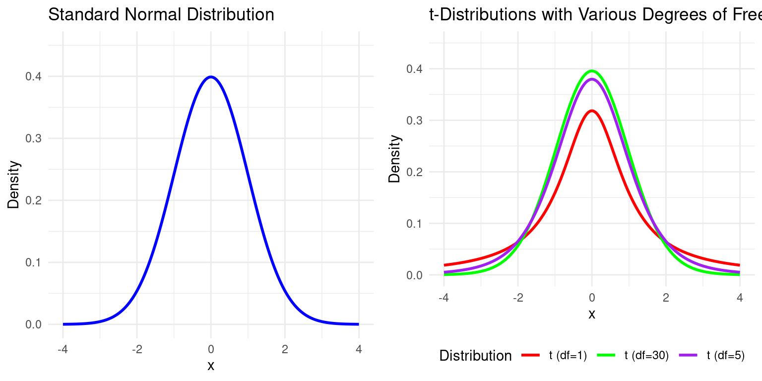
- The t-distribution looks very similar to the normal distribution but has “fatter tails,” reflecting the added uncertainty from estimating \(\sigma^2\).
- It is characterized by its degrees of freedom (df), which for Simple Linear Regression is \(df = n - 2\).
- As the sample size (\(n\)) gets large, the t-distribution converges to the standard normal distribution.
Visualization
Example: \(t\)-distribution vs. Normal Distribution
Example: A \(t\)-test in Simple Linear Regression
Example: \(t\)-test in Linear Regression
Consider the following regression output:
Code
summary(slr_model)
##
## Call:
## lm(formula = wage ~ educ, data = dat)
##
## Residuals:
##     Min      1Q  Median      3Q     Max
## -6.7201 -2.3878 -0.3926  1.9554 11.6092
##
## Coefficients:
##             Estimate Std. Error t value Pr(>|t|)
## (Intercept)   1.7863     2.5164   0.710    0.479
## educ          1.1498     0.1887   6.092 2.19e-08 ***
## ---
## Signif. codes:  0 '***' 0.001 '**' 0.01 '*' 0.05 '.' 0.1 ' ' 1
##
## Residual standard error: 3.4 on 98 degrees of freedom
## Multiple R-squared:  0.2747, Adjusted R-squared:  0.2673
## F-statistic: 37.11 on 1 and 98 DF,  p-value: 2.192e-08
From this, we can see that the regression standard error (SER), \(\hat{\sigma} = 3.4\). We can also see that the SE on the educ coefficient is 0.19. We can relate the two by dividing SER by \(\sqrt{\sum (X_i - \bar{X})^2}\):
We can therefore manually calculate the \(t\)-statistic testing \(H_0: \beta=0\) as:
Finally we can even calculate the two-sided \(p\)-value of observing a test statistic this extreme under the null hypothesis:
What did we do?
- The Linear Model’s Purpose:
- Econometrics uses the linear regression model to estimate the relationship between a dependent variable (e.g., wage) and one or more explanatory variables (e.g., education). The goal is to estimate an unknown “population” relationship using a “sample” of data.
- The OLS Method:
- The model’s coefficients (slope and intercept) are estimated using the Ordinary Least Squares (OLS) method. This technique finds the best-fitting line by minimizing the sum of the squared differences (residuals) between the actual data points and the predicted values on the line.
- Interpretation of Coefficients:
- The meaning of a coefficient depends on the model’s structure. While a basic model shows unit changes, using logarithms (log-level, level-log, log-log) allows for interpreting relationships in terms of percentage changes or elasticities, which is common in economics.
The End
![]()
Empirical Economics: Lecture 1 - The Linear Model I