Empirical Economics
Lecture 2: The Linear Model II
Outline
Course Overview
- Linear Model I
- Linear Model II
- Time Series and Prediction
- Panel Data I
- Panel Data II
- Binary Outcome Data
- Potential Outcomes and Difference-in-differences
- Instrumental Variables
What do we do today?
First two lectures devoted to the linear model.
Prequisite knowledge:
- How do we model the processes that might have generated our data?
- How do we summarize and describe data, and try to uncover what process may have generated it?
- Probability and statistics
This lecture:
- Multiple linear regression, hypotheses tests, F-tests, Interactions, Understanding Statistical Output
Material: Wooldridge Chapters 3 and 4
Multiple Regression
Introduction to Multiple Linear Regression
Simple Linear Regression is often inadequate because we can’t control for other factors that might be important. This leads to omitted variable bias.
The solution is to include those other factors in the model.
Definition: Multiple Linear Regression Model
\[ y = \beta_0 + \beta_1 x_1 + \beta_2 x_2 + ... + \beta_k x_k + u \]
Now we have \(k\) explanatory variables.
- \(\beta_j\) is the effect of a one-unit change in \(x_j\) on \(y\), holding all other explanatory variables (\(x_1, ..., x_{j-1}, x_{j+1}, ... x_k\)) constant.
- This is the concept of ceteris paribus (all else equal). MLR allows us to isolate the effect of one variable while mathematically controlling for the others.
OLS Estimation in MLR
The principle is the same: we choose \(\hat{\beta}_0, \hat{\beta}_1, ..., \hat{\beta}_k\) to minimize the Sum of Squared Residuals (SSR).
The formulas are complex (usually done with matrix algebra) but are easily handled by software:
lm(y ~ x1 + x2, data=df)in Rreg y x1 x2in Statapf.feols("y ~ x1 + x2", data=df)afterimport pyfixest as pfin Python.1
Interpretation of MLR
In multiple linear regression, our primary goal is often to estimate the causal effect of a specific variable of interest (say \(X_1\)) on an outcome (\(Y\)). The challenge is that in the real world, many factors are changing at once.
The purpose of control variables (\(X_2, X_3, \dots\)) is to statistically “hold constant” other relevant factors that could be confounding our results.
The validity of your estimated causal effect hinges on choosing the right controls. Including the wrong ones can be worse than including none at all.
Good vs. Bad Controls
- A good control variable is a confounder. A confounder is a pre-treatment variable that is correlated with both your variable of interest (\(X_1\)) and your outcome (\(Y\)).
- Failing to control for a confounder leads to omitted variable bias (OVB). The coefficient \(\beta_1\) will incorrectly absorb the effect of the missing variable.
Example: Good Control Variable
In estimating the effect of education (\(X_1\)) on wages (\(Y\)), innate ability is a classic confounder. Ability is likely correlated with how much education someone pursues and their potential earnings.
Controlling for a proxy of ability (like an IQ test score, \(X_2\)) helps to prevent the estimated return to education from being biased upwards.
Bad Controls
- Bad controls are variables that, when included in a regression, actually induce bias or obscure the true causal relationship. There are two kinds of them:
- An intermediate variable that lies on the causal pathway between your variable of interest and the outcome.
- Controlling for a mediator closes off one of the channels through which \(X_1\) affects \(Y\). You are essentially holding constant a part of the effect you want to measure.
- A collider variable that is causally influenced by both the variable of interest (\(X_1\)) and the outcome (\(Y\)).
- Controlling for a collider can induce a spurious statistical association between \(X_1\) and \(Y\), even if none exists.
- An intermediate variable that lies on the causal pathway between your variable of interest and the outcome.
Example: Bad Control
Suppose we study the relationship between having a MSc degree (\(X_1\)) and having a start-up idea (\(Y\)) among people who receive research grants (\(Z\)). Getting a grant (\(Z\)) may be caused by both having a MSc and having a good idea.
If we only look at people who received grants (i.e., control for \(Z\)), we might find a spurious negative correlation. Within the grant-recipient pool, someone with a MSc but a weak idea could get the grant, as could someone without a MSc but a brilliant idea. This creates an artificial trade-off in our selected sample.
Variance of OLS Estimators in MLR
Definition: (Estimated) Variance of the OLS Estimator (Multivariate)
\[ \widehat{Var}(\hat{\beta}_j) = \frac{\hat{\sigma}^2}{SST_j (1 - R_j^2)} \]
- \(SST_j\) is the total variation in \(x_j\): \(\sum_{i=1}^N (x_{ij} - \bar{x}_j)^2\)
- \(R_j^2\) is the R-squared from a regression of \(x_j\) on all other explanatory variables in the model.
- The variance of a coefficient \(\hat{\beta}_j\) now depends on multicollinearity – how correlated \(x_j\) is with the other explanatory variables.
- If \(x_j\) is highly correlated with other \(x\)’s, \(R_j^2\) will be close to 1, making the denominator small and \(Var(\hat{\beta}_j)\) very large. This is imperfect multicollinearity.
- The no perfect collinearity assumption for MLR means that no \(x_j\) can be a perfect linear combination of the others (i.e., \(R_j^2 \neq 1\)).
Hypothesis Testing in Multiple Regression
- Once we’ve estimated our model, \(\widehat{y} = \hat{\beta}_0 + \hat{\beta}_1 x_1 + \dots + \hat{\beta}_k x_k\), we need to ask: Is the relationship we found statistically significant?
- Our estimates \(\hat{\beta}_0\) and \(\hat{\beta}_j\) are based on a sample of data. They are subject to sampling variability.
- It’s possible that the true relationship in the population is zero (\(\beta_1 = 0\)), and we just found a non-zero \(\hat{\beta}_1\) by random chance.
- In addition to the \(t\)-test, introduced with the Simple Linear Regression model, we also have the \(F\)-test:
- This tests the joint significance of multiple coefficients or the model as a whole.
The \(t\)-Test: Significance of a Single Coefficient
- The \(t\)-test is our tool for testing a hypothesis about a single coefficient.
- The most common hypothesis is that a variable has no effect on the dependent variable.
- Hypotheses for a single coefficient \(\beta_j\):
- Null Hypothesis (\(H_0\)): The variable has no effect. \(H_0: \beta_j = 0\)
- Alternative Hypothesis (\(H_A\)): The variable does have an effect. \(H_A: \beta_j \neq 0\)
- We calculate the t-statistic, which measures how many standard errors our estimated coefficient is away from the hypothesized value (zero).
The \(t\)-statistic (Multivariate)
\[ t = \frac{\text{Estimate} - \text{Hypothesized Value}}{\text{Standard Error}} = \frac{\hat{\beta}_j - 0}{se(\hat{\beta}_j)} \]
where the \(se(\hat{\beta}_j)\) is the square root of \(Var(\hat{\beta}_j)\) as presented earlier.
The F-Test: Testing Joint Significance
- The F-test is used to test hypotheses about multiple coefficients at the same time.
- Its most common use is to test the overall significance of the regression model.
F Test for Overall Significance
This tests whether any of our independent variables have an effect on the dependent variable.
Model: \(y = \beta_0 + \beta_1 x_1 + \beta_2 x_2 + \dots + \beta_k x_k + u\)
Null Hypothesis (\(H_0\)): None of the independent variables have an effect on \(y\). The model has no explanatory power. \(H_0: \beta_1 = \beta_2 = \dots = \beta_k = 0\)
Alternative Hypothesis (\(H_A\)): \(H_0\) not true.
- At least one of the coefficients is not zero. The model has some explanatory power.
F-statistic
- In general, the F-test serves to compare a “restricted model”, where some of the \(\beta\) coefficients are zero under a null hypothesis, against an “unrestricted” model where coefficients are allowed to vary.
- A large F-statistic suggests that the unrestricted model explains significantly more variation in \(y\) than the restricted model.
- Like the t-test, we typically look at the p-value for the F-statistic. If \(p < 0.05\), we reject the null and conclude our model is jointly significant.
F-statistic Procedure
F Statistic: Definition (General)
The F statistic is defined as:
\[ F = \frac{(SSR_{restricted} - SSR_{unrestricted}) / q}{SSR_{unrestricted} / (n - k - 1)} \]
Where:
- \(SSR_{restricted}\) = Sum of Squared Residuals from the restricted model (the model with fewer predictors, where the null hypothesis is assumed to be true).
- \(SSR_{unrestricted}\) = Sum of Squared Residuals from the unrestricted model (the model with more predictors).
- \(q\) = The number of restrictions being tested. This is essentially the number of parameters that are set to zero in the restricted model. You can often simply count the number of equals signs in your null hypothesis to determine the value of q. For instance, if your null hypothesis is \(H_0: \beta_1 = \beta_2 = 0\), then \(q=2\) because you are imposing two restrictions.
- \(n\) = The number of observations in your sample.
- \(k\) = The number of parameters in the unrestricted model (including the intercept).
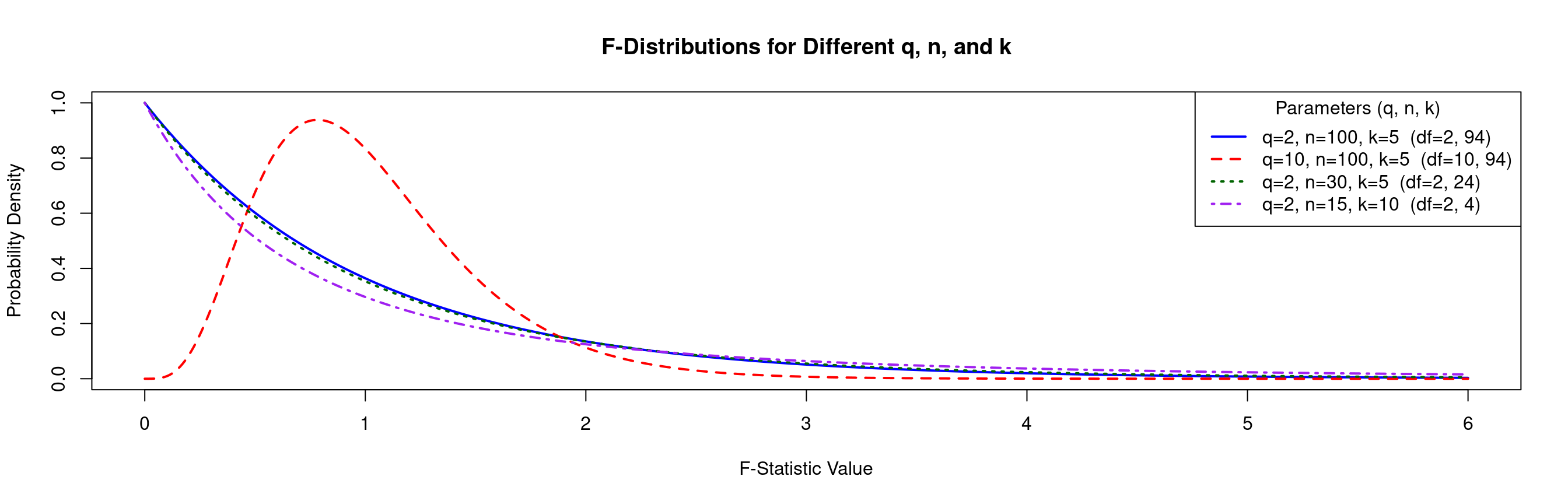
F Distribution: Visualization
- The \(F\) distribution comes with three parameters, \(n\), \(k\) and \(q\) as defined in the previous slide.
Example: F Distribution
Summary: \(t\)-test vs. \(F\)-test
- It’s crucial to understand when to use each test.
- A group of variables can be jointly significant (F-test) even if no single variable is individually significant (t-tests).
| Feature | t-test | F-test |
|---|---|---|
| Scope | One coefficient at a time | Two or more coefficients at a time |
| Typical Use | Is this specific variable significant? | Is this group of variables jointly significant? OR Is the model as a whole useful? |
| Null Hypothesis | \(H_0: \beta_j = 0\) | \(H_0: \beta_1 = \beta_2 = \dots = 0\) |
| Test Statistic | \(t = \frac{\hat{\beta}_j}{se(\hat{\beta}_j)}\) | Compares Restricted vs. Unrestricted sum of squares |
| Key Question | “Does education significantly affect wage, holding other factors constant?” | “Does a person’s work experience, measured by exper and exper^2, jointly affect their wage?” |
Interactions and Dummies in MLR
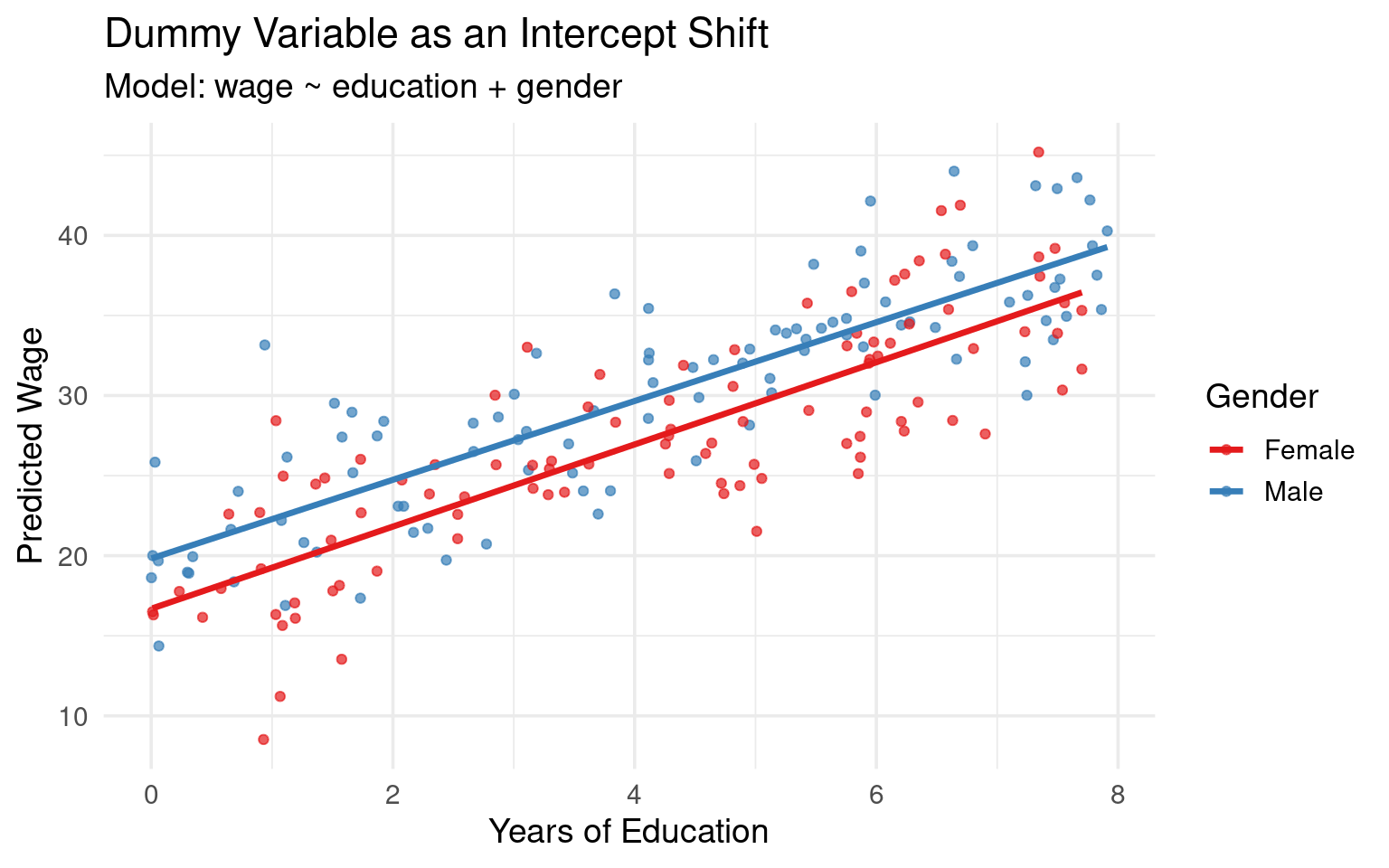
Dummies in Multiple Regression
The power of dummy variables becomes clear when we add other regressors. Let’s add years of education (
Educ) to our model:\[ Wage_i = \beta_0 + \beta_1 Female_i + \beta_2 Educ_i + u_i \]
We again analyze the regression equation for each group, now holding
Educconstant.- For Males (\(Female_i = 0\)):
- \(E[Wage_i | Female_i=0, Educ_i] = \beta_0 + \beta_2 Educ_i\)
- This is the wage-education profile for males. It’s a line with intercept \(\beta_0\) and slope \(\beta_2\).
- For Females (\(Female_i = 1\)):
- \(E[Wage_i | Female_i=1, Educ_i] = \beta_0 + \beta_1(1) + \beta_2 Educ_i = (\beta_0 + \beta_1) + \beta_2 Educ_i\)
- This is the wage-education profile for females. It’s a line with a different intercept, \((\beta_0 + \beta_1)\), but the same slope, \(\beta_2\).
- For Males (\(Female_i = 0\)):
Reinterpreting Dummies
- \(\beta_0\): The intercept for the reference group (males). It is the predicted wage for a male with zero years of education.
- \(\beta_1\): The difference in the intercept between females and males. It is the predicted wage difference between a female and a male who have the same level of education.
- \(\beta_2\): The slope of the wage-education profile. It represents the change in wage for an additional year of education, and this model constrains that effect to be the same for both men and women.
Visualization
- Graphical Intuition: This model generates two parallel regression lines. They have the same slope (\(\beta_2\)), but are separated vertically by a distance of \(\beta_1\).
Interaction Effects
The standard linear regression model \(\text{Wage}_i = \beta_0 + \beta_1 \text{Gender}_i + \beta_2 \text{Educ}_i + u_i\) assumes the effect of education on wages (\(\beta_2\)) is identical for men and women.
What if an extra year of education has a different return for females than for males? To allow for this, we must let the slope differ between the groups. We do this by adding an interaction term.
The interaction term is simply the product of the dummy variable and the continuous variable. \(Wage_i = \beta_0 + \beta_1 Female_i + \beta_2 Educ_i + \beta_3 (Female_i \cdot Educ_i) + u_i\)
Once more, we derive the regression line for each group.
- For Males (\(Female_i = 0\)): The dummy and interaction term are both zero.
- \(E[Wage_i | Female_i=0, Educ_i] = \beta_0 + \beta_2 Educ_i\)
- The intercept is \(\beta_0\) and the slope is \(\beta_2\). This is the baseline profile.
- For Females (\(Female_i = 1\)):
- \(E[Wage_i | Female_i=1, Educ_i] = \beta_0 + \beta_1(1) + \beta_2 Educ_i + \beta_3 (1 \cdot Educ_i)\)
- Group the terms by the constant and the variable
Educ: - \(E[Wage_i | Female_i=1, Educ_i] = (\beta_0 + \beta_1) + (\beta_2 + \beta_3) Educ_i\)
- For females, the intercept is \((\beta_0 + \beta_1)\) and the slope is \((\beta_2 + \beta_3)\).
- For Males (\(Female_i = 0\)): The dummy and interaction term are both zero.
Interpreting Interaction Terms
The interpretation of the “main effects” (\(\beta_1\) and \(\beta_2\)) changes fundamentally when an interaction term is present.
\(\beta_2\) is the effect of an additional year of education on wages for the reference group (males) only.
\(\beta_1\) is the difference in expected wages between females and males when
Educ= 0. This is the difference in the intercepts. This coefficient is often not meaningful on its own ifEduc=0is not a relevant value in the data.\(\beta_3\) (Interaction Coefficient) is the difference in the slopes between males and females. It measures by how much the effect of an additional year of education differs for females compared to males. This is often the coefficient of primary interest.
Hence, the effect of
EduconWagefor men is \(\beta_2\), and \(\beta_2 + \beta_3\) for women.
Visualization
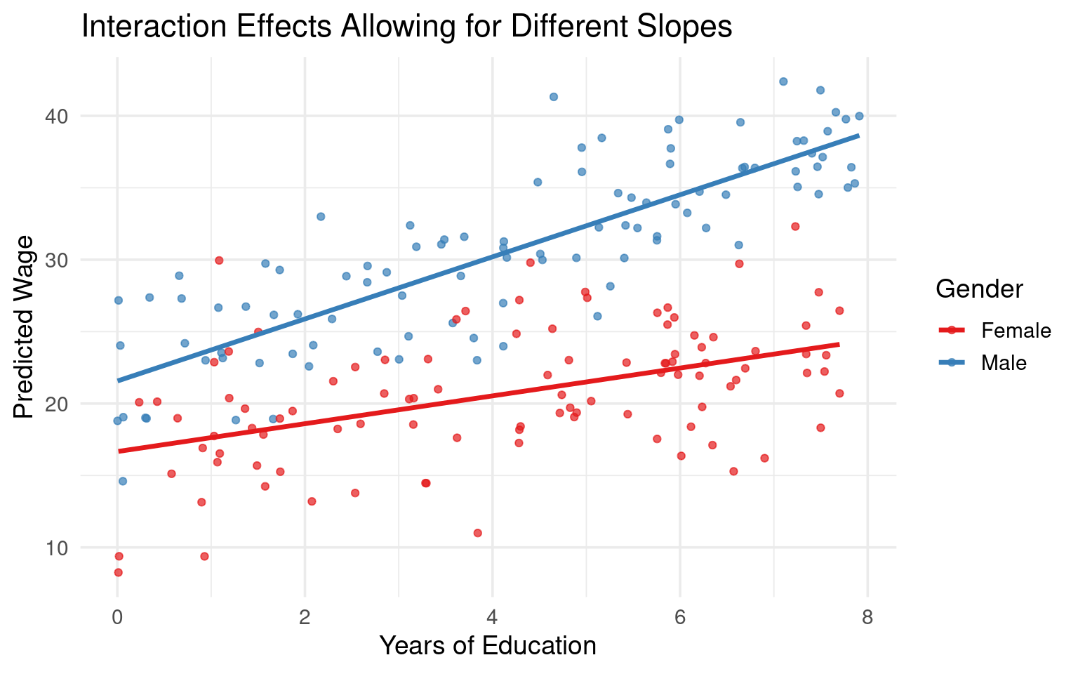
Total Effect Under Interaction
- The effect of a variable is no longer a single coefficient but may be a function of another variable.
Example: Education Gender Interaction
The marginal effect of Education for Females is: \(\frac{\partial E[wage_i | Female_i=1, Educ_i]}{\partial Educ_i} = \beta_2 + \beta_3\)
The wage differential between Females and Males is: \(E[wage|F=1] - E[wage|F=0] = ((\beta_0 + \beta_1) + (\beta_2 + \beta_3)Educ_i) - (\beta_0 + \beta_2 Educ_i) = \beta_1 + \beta_3 Educ_i\). The wage gap is no longer constant; it depends on the level of education.
- Hypothesis Testing:
- To test if education has a different effect for females, the null hypothesis is \(H_0: \beta_3 = 0\).
- To test if gender has any effect on wages at all, you must test if the lines are identical, which requires a joint test: \(H_0: \beta_1 = 0 \text{ and } \beta_3 = 0\). This is done with an F-test.
Multiple Categories
- Suppose now you have a categorical variable with k distinct categories (e.g., region, with categories North, South, East, West).
- You cannot simply code this as 1, 2, 3, 4 because that would impose a nonsensical ordered relationship.
- To properly include this information in a regression, you must create k-1 binary (or “dummy”) variables.
- Each dummy variable represents one of the categories.
- An observation will have a value of 1 for the dummy variable corresponding to its category, and 0 for all other dummy variables.
- The Dummy Variable Trap
- You must always omit one category, which becomes the baseline or reference category. If you were to include a dummy variable for every category, you would fall into the “dummy variable trap.”
- This is a situation of perfect multicollinearity, where one dummy variable can be perfectly predicted by the others.
Example Model
- For example, if you know an observation is not in the North, South, or East, it must be in the West.
- This redundancy makes it impossible for the model to estimate the individual effect of each category.
Example: Multiple Dummies with Reference Category
With “West” as the baseline, the model would be:
\[ y_i = \beta_0 + \beta_1 \text{North}_i + \beta_2 \text{South}_i + \beta_3 \text{East}_i + \dots + u_i \]
Where:
- \(\text{North}_i = 1\) if the observation is in the North, 0 otherwise.
- \(\text{South}_i = 1\) if the observation is in the South, 0 otherwise.
- \(\text{East}_i = 1\) if the observation is in the East, 0 otherwise.
Interpretation of the Coefficients
The Intercept (\(\beta_0\)) now represents the average value of the dependent variable for the baseline category (the one you omitted).
- In our example, it would be the average value of \(y\) for the “West” region, assuming all other independent variables in the model are zero.
The Dummy Coefficients (\(\beta_1, \beta_2, \dots\)): Each dummy variable’s coefficient represents the average difference in the dependent variable between that category and the baseline category, holding all other variables constant.
- \(\beta_1\): Represents the average difference in \(y\) between the “North” region and the “West” region.
- \(\beta_2\): Represents the average difference in \(y\) between the “South” region and the “West” region.
- \(\beta_3\): Represents the average difference in \(y\) between the “East” region and the “West” region.
The coefficients do not show the average value of \(y\) for that category directly. They show the difference relative to the baseline.
Statistical Significance: If the \(p\)-value for a dummy variable’s coefficient is statistically significant, it suggests that there is a meaningful difference in the outcome variable between that category and the baseline category.
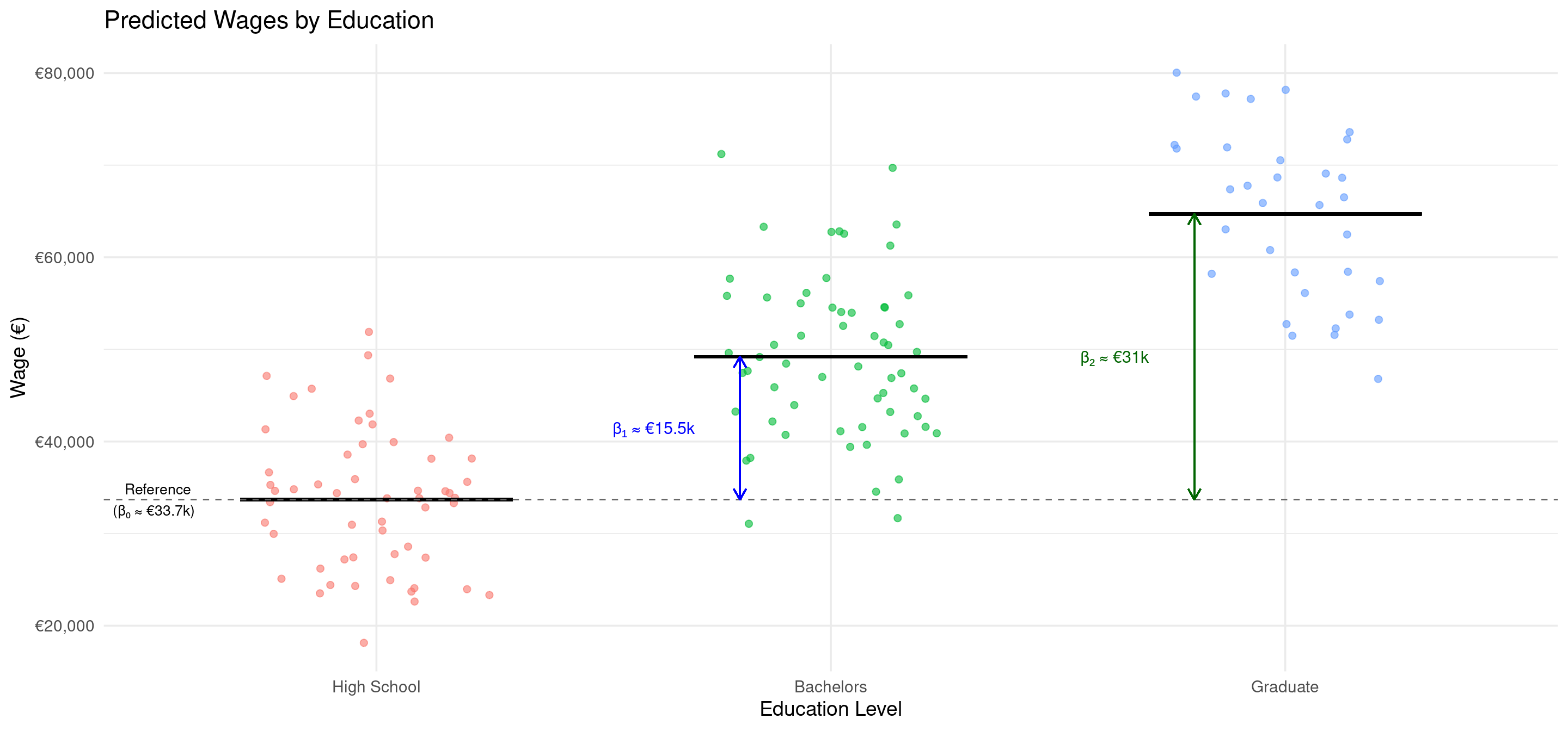
Example: Predicting Wages
Scenario: We want to predict an individual’s wage based on their education level, which we have categorized as “High School,” “Bachelors,” and “Masters” We will use “High School” as our baseline category.
\[ \text{Wage}_i = \beta_0 + \beta_1 \text{Bachelors}_i + \beta_2 \text{Masters}_i + u_i \]
Let’s say we run the regression and get the following results: \[ \widehat{\text{Wage}}_i = 35000 + 15000 \cdot \text{Bachelors}_i + 30000 \cdot \text{Masters}_i \]
Interpretation:
- \(\hat{\beta}_0 = €35000\): The average wage for an individual with a “High School” education (the baseline) is €35,000.
- \(\hat{\beta}_1 = €15000\): On average, individuals with a “Bachelors” degree earn €15,000 more than those with a “High School” education. The predicted average wage for this group is €35,000 + €15,000 = €50,000.
- \(\hat{\beta}_2 = €30000\): On average, individuals with a “Graduate” degree earn €30,000 more than those with a “High School” education. The predicted average wage for this group is €35,000 + €30,000 = €65,000.
Changing Baseline
While your choice of a baseline category changes the interpretation of the individual coefficients, it does not change the overall significance of the categorical variable as a whole.
When you include a set of dummy variables for a single categorical predictor (e.g., “Bachelors” and “Graduate” for the “Education” variable), the F-statistic tests the joint null hypothesis that all of these dummy coefficients are equal to zero.
- \(H_0: \beta_{\text{Bachelors}} = 0 \text{ AND } \beta_{\text{Graduate}} = 0\)
- In words: The F-test checks if the “Education” variable, as a whole, has any explanatory power.
Why it is invariant: The overall fit of the model (e.g., the R-squared) remains identical regardless of which category you choose as the baseline.
- You are using the same information and explaining the same amount of variation in the dependent variable. Since the F-statistic is calculated based on this overall model fit, its value does not change.
- The conclusion about whether “Education” is a significant predictor will be the same no matter which level is your reference.
Interpretation of Parameters
While the F-test looks at the variable as a whole, the t-test for each individual dummy coefficient examines a more specific comparison.
Each dummy coefficient (\(\beta_j\)) represents the estimated average difference in the outcome variable between category j and the baseline category.
- The t-test: The t-test for a specific coefficient tests whether this difference is statistically significant (i.e., different from zero).
- Null Hypothesis (\(H_0: \beta_j = 0\)): The average outcome for category j is the same as the average outcome for the baseline category.
- Alternative Hypothesis (\(H_a: \beta_j \neq 0\)): There is a statistically significant difference in the average outcome between category j and the baseline category.
Example: In our wage regression, the t-test for \(\beta_{\text{Bachelors}}\) answers the question: “Is the average wage for people with a Bachelor’s degree significantly different from the average wage for people with a High School diploma (the baseline)?”
Illustration
Understanding Statistical Output
Understanding Statistical Output
- By now, we can understand virtually all of the standard statistical output from R/Python/Stata.
- Let’s look at the full output from R/Python/Stata for our simple regression.
Code
mlr_model <- lm(wage ~ educ + exper, data = dat_mlr)
summary(mlr_model)
##
## Call:
## lm(formula = wage ~ educ + exper, data = dat_mlr)
##
## Residuals:
##     Min      1Q  Median      3Q     Max
## -7.3544 -1.9212  0.1218  2.1522  7.5290
##
## Coefficients:
##             Estimate Std. Error t value Pr(>|t|)
## (Intercept)  2.82941    2.64978   1.068   0.2883
## educ         1.02959    0.17534   5.872 6.03e-08 ***
## exper        0.16733    0.06647   2.518   0.0135 *
## ---
## Signif. codes:  0 '***' 0.001 '**' 0.01 '*' 0.05 '.' 0.1 ' ' 1
##
## Residual standard error: 3.142 on 97 degrees of freedom
## Multiple R-squared:  0.2825, Adjusted R-squared:  0.2677
## F-statistic:  19.1 on 2 and 97 DF,  p-value: 1.016e-07
Code
import statsmodels.api as sm
import pandas as pd
# Create a DataFrame for X (automatically keeps variable names)
X = pd.DataFrame({
    'educ': r.dat_mlr['educ'],
    'exper': r.dat_mlr['exper']
})

X = sm.add_constant(X)  # Adds 'const' column
y = r.dat_mlr['wage']
model = sm.OLS(y, X).fit()
print(model.summary())
##                             OLS Regression Results
## ==============================================================================
## Dep. Variable:                   wage   R-squared:                       0.283
## Model:                            OLS   Adj. R-squared:                  0.268
## Method:                 Least Squares   F-statistic:                     19.10
## Date:                Wed, 29 Oct 2025   Prob (F-statistic):           1.02e-07
## Time:                        12:56:16   Log-Likelihood:                -254.87
## No. Observations:                 100   AIC:                             515.7
## Df Residuals:                      97   BIC:                             523.6
## Df Model:                           2
## Covariance Type:            nonrobust
## ==============================================================================
##                  coef    std err          t      P>|t|      [0.025      0.975]
## ------------------------------------------------------------------------------
## const          2.8294      2.650      1.068      0.288      -2.430       8.088
## educ           1.0296      0.175      5.872      0.000       0.682       1.378
## exper          0.1673      0.066      2.518      0.013       0.035       0.299
## ==============================================================================
## Omnibus:                        0.187   Durbin-Watson:                   2.158
## Prob(Omnibus):                  0.911   Jarque-Bera (JB):                0.359
## Skew:                          -0.059   Prob(JB):                        0.836
## Kurtosis:                       2.731   Cond. No.                         175.
## ==============================================================================
##
## Notes:
## [1] Standard Errors assume that the covariance matrix of the errors is correctly specified.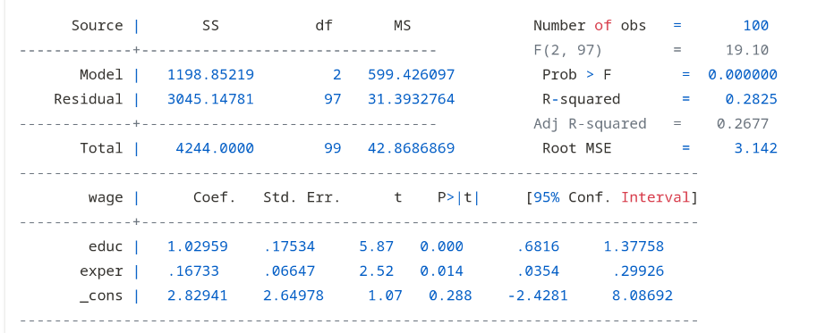
Understanding Statistical Output (Cont.)
- Coefficients:
Estimateorcoef: These are \(\hat{\beta}_0\) (Intercept), \(\hat{\beta}_1\) (educ) and \(\hat{\beta}_2\) (exper).Std. Error: The standard errors of the estimates, \(se(\hat{\beta}_j)\), which measure their sampling uncertainty.t value: The t-statistic used for hypothesis testing (Estimate/Std. Error).Pr(>|t|): The p-value for the t-test.
- Goodness-of-Fit:
Residual standard error(R only): This is the SER (3.14).R-squared: This is our R-squared (0.27). The model explains about 28% of the variation in wages.
Interpretation with Controls
- Important: we can only interpret the coefficients that are statistically distinguishable from zero.
- The t-statistics tell us whether that is the case.
Educ: \(\hat{\beta}_1 \approx 1.02\): Holding experience constant, one more year of education is associated with a €1.02/hr increase in wages, on average.Exper: \(\hat{\beta}_2 \approx 0.16\): Holding education constant, one more year of experience is associated with a €0.16/hr increase in wages, on average.- The R-squared increased relative to the simple model, suggesting this model explains more variation in wages.
Robust Standard Errors
OLS Variance
Our goal is to find the variance of the OLS estimator, \(Var(\hat{\beta}_1)\), which is the basis for all statistical inference. Conditional on the regressors \(x_i\), we have:1
\[ Var(\hat{\beta}_1) = \frac{1}{\left(\sum (x_i - \bar{x})^2\right)^2} Var\left(\sum_{i=1}^N (x_i - \bar{x})u_i\right) \]
To evaluate the variance of the sum, we must make assumptions about the error terms, \(u_i\). The standard output in R/Python/Stata imposes two key assumptions on the errors:
- The errors are uncorrelated across observations. Mathematically, \(Cov(u_i, u_j) = 0\) for all \(i \neq j\).
- Homoskedasticity: The errors have a constant variance. Mathematically, \(Var(u_i) = \sigma^2\) for all \(i\).
The Problem of Heteroskedasticity
Under homoskedasticity, the variance of \(\hat{\beta_1}\) equals:
\[ Var(\hat{\beta}_1) = \frac{\sigma^2 \sum (x_i - \bar{x})^2}{\left(\sum (x_i - \bar{x})^2\right)^2} = \frac{\sigma^2}{\sum (x_i - \bar{x})^2} \]
The assumption of homoskedasticity (“same scatter”) is often violated in economic data.
Heteroskedasticity occurs if the variance of the error term is not constant across observations.
If we ignore this and use the classical formula, our inference can be severely misleading.
HC Robust SE’s
Formal Definition: \(Var(u_i) = \sigma_i^2\). The variance is indexed by
i, meaning it can take on a different value for each observation.Example: Consider a regression of household food expenditure on household income. Low-income households have limited budgets, so their food spending will be tightly clustered around a certain amount (low variance). High-income households have more discretion; some may spend a lot on gourmet food while others spend relatively little, leading to a much wider spread of data points (high variance). The variance of the error term, which captures this deviation from the average, increases with income.
Under heteroskedasticity, the HC-Robust variance equals:
\[ Var(\hat{\beta}_1) = \frac{\sum_{i=1}^N (x_i - \bar{x})^2 \sigma_i^2}{\left(\sum_{i=1}^N (x_i - \bar{x})^2\right)^2} \]
This is the true variance of the OLS estimator in the presence of heteroskedasticity.
Estimation of HC Standard Error
The challenge is that we cannot compute the true variance because we do not know the individual error variances, \(\sigma_i^2\).
The insight (White, 1980) is to use the squared OLS residual for each observation, \(\hat{u}_i^2 = (y_i - \hat{y}_i)^2\), as an estimator for the unobserved error variance, \(\sigma_i^2\).
We construct the estimator by taking the correct formula for the variance and “plugging in” \(\hat{u}_i^2\) for \(\sigma_i^2\). This gives the heteroskedasticity-robust variance estimator, also alled the White estimator or HC estimator:
\[ \widehat{Var}_{HC}(\hat{\beta}_1) = \frac{\sum_{i=1}^N (x_i - \bar{x})^2 \hat{u}_i^2}{\left(\sum_{i=1}^N (x_i - \bar{x})^2\right)^2} \]
The square root of this value is the heteroskedasticity-robust standard error (or HC-robust SE).
This is a consistent estimator of the standard error. It only works for large \(n\).
HC Robust Standard Errors in Software
- By default, you should estimate a regression and compute heteroskedastic standard errors.
- Because this is not the default behavior in statistical packages, you need to do that manually.
- In R:
feols(y ~ x1 + x2, data = df, vcov='hc1') - In Python:
pf.feols("y ~ x1 + x2", data = df).vcov("HC1") - In Stata:
reg y x1 x2, robust
- In R:
Summary HC Robust SE
- What it corrects for:
- HC-robust standard errors correct for heteroskedasticity. They do not correct for serial correlation (which requires clustered SEs) or omitted variable bias.
- When to use:
- In cross-sectional data analysis, heteroskedasticity is the rule rather than the exception. The modern consensus among econometricians is to use HC-robust standard errors by default.
- The cost of using them if errors are truly homoskedastic is minimal in large samples, while the cost of failing to use them if heteroskedasticity is present is high (invalid inference).
- Efficiency:
- It’s crucial to remember that OLS is still unbiased and consistent under heteroskedasticity. However, it is not efficient. HC-robust standard errors fix the inference (t-tests, p-values), but they do not make the OLS estimator itself more efficient. For that, you would need a different estimation method like Weighted Least Squares (WLS).
Clustered Standard Errors
Intra-Cluster Correlation
In many economic datasets, the assumption that \(Cov(u_i, u_j) = 0\) is unrealistic.
Examples are students nested within schools, individuals within states, or firms over time (panel data).
Unobserved factors at the group level can induce correlation among the error terms within that group.
This structure is called clustered data.
Notation Clustered SE’s
Let’s introduce notation for clusters. Let \(g\) index the cluster (e.g., a school) and \(i\) index the individual within the cluster. An observation is denoted by \(gi\). Our model is now:
\[ y_{gi} = \beta_0 + \beta_1 x_{gi} + u_{gi} \]
The key feature of clustered data is the assumed error structure:
- \(Cov(u_{gi}, u_{gj}) \neq 0\) for \(i \neq j\) (Correlation within a cluster \(g\))
- \(Cov(u_{gi}, u_{g'j}) = 0\) for \(g \neq g'\) (No correlation between clusters)
If we ignore this structure and use the standard OLS formula, we are incorrectly zeroing out all the covariance terms in the variance calculation.
- If these covariance terms are, on average, positive (which is common), we will systematically underestimate the true variance of \(\hat{\beta}_1\). This leads to standard errors that are too small.
Clustering SE’s
- Clustered Standard Errors are approximately calculated as follows:1
Procedure Clustered Standard Errors
- First, run the OLS regression as usual to obtain the coefficient estimates (\(\hat{\beta}\)) and the residuals (\(u_{gi}\)).
- Next, group the residuals by cluster.
- For each cluster, calculate a term that incorporates the variance and covariance of the residuals within that cluster. This step explicitly captures the \(Cov(u_{gi}, u_{gj})\) terms that standard OLS ignores.
- Sum these terms across all the clusters to arrive at an “updated” variance estimate.
- This process effectively treats each cluster as a single, larger observation.
- By summing up the information from each cluster, we are allowing for the errors to be correlated inside the cluster, but maintaining the assumption that they are independent across different clusters.
- If observations within a cluster provide very similar information, the cluster as a whole contributes less “unique” information than if the observations were all independent. This typically results in larger, more conservative standard errors.
When to Cluster
- When to Cluster:
- Cluster standard errors if you suspect the error terms are correlated within groups. This is common with panel data, data from multi-stage surveys, or if a policy is applied at a group level (e.g., a state-level law).
- What Level to Cluster at:
- You should cluster at the level at which the unobserved components are shared. If you have students in classrooms within schools, and you suspect shocks at both the classroom and school level, you should cluster at the broader level (school), as this allows for correlation within classrooms and between classrooms within the same school.
- Consequences of Failure to Cluster:
- If intra-cluster correlation exists and you use standard OLS standard errors, your standard errors will be biased downwards. This will make you overly confident in your results and lead to spurious findings of statistical significance.
Clustering in Software
- Similarly to HC-Robust standard errors, clustered standard errors need to be applied explicitly in statistical software.
- In R:
feols(y ~ x1 + x2, data = df, vcov=~cluster_variable) - In Python:
pf.feols("y ~ x1 + x2", data = df).vcov({"CRV3": "cluster_variable"}).summary() - In Stata:
reg y x1 x2, vce(cluster cluster_variable)
- In R:
Summary
What did we do?
- Multiple Linear Regression:
- We introduced the method of multiple linear regression and provided ourselves with an interpretation of the estimated coefficients.
- Control Variables:
- For OLS estimates to be unbiased (correct on average), a set of classical assumptions must hold. The most critical is the Zero Conditional Mean assumption, which states that unobserved factors (like innate ability) must not be correlated with the explanatory variable (like education). We discussed the logic of inclusion of control variables to minimize this kind of bias.
- Hypothesis Testing:
- After estimating a model, we use hypothesis testing to determine if the results are statistically significant.
- The t-test is used to assess the significance of a single variable, while the F-test is used to assess the joint significance of multiple variables or the overall explanatory power of the model.
What did we do? (Cont.)
- Dummies and Interactions:
- We discussed the interpretation of dummy variables and interaction terms in a multiple linear regression context.
- Standard errors of estimated regression parameters:
- We discussed the issue of standard errors in regression. We saw that the standard errors statistical software computes by default are almost certainly incorrect. We saw two alternatives, the HC-robust standard error and the Cluster-robust standard error, and focused on their estimation.
The End
Appendix 1: Cluster-robust SEs
Expressing the Variance
We now express the variance of the OLS estimator, \(Var(\hat{\beta}_1)\) in a form recognizing the cluster structure:
\[ \begin{align} Var(\hat{\beta}_1) &= Var \left( \beta_1 + \frac{\sum_{i=1}^N (x_i - \bar{x})u_i}{\sum_{i=1}^N (x_i - \bar{x})^2} \right) \\ &= \frac{1}{\left(\sum (x_i - \bar{x})^2\right)^2} Var\left(\sum_{i=1}^N (x_i - \bar{x})u_i\right) \\ &= \frac{1}{\left(\sum (x_i - \bar{x})^2\right)^2} {Var\left(\sum_{g=1}^G \sum_{i=1}^{N_g} (x_{gi} - \bar{x})u_{gi}\right)} \end{align} \]
In the final equality, we recognize that the sum over all observations can be partitioned into the sum over all observations within one cluster (from \(i\) to \(N_g\)), and then summing over each cluster (from \(g=1\) to \(G\)).
Deriving the Cluster-Robust Variance
Restating the result from the previous slide:
\[ Var(\hat{\beta}_1) = \frac{1}{\left(\sum_{g,i} (x_{gi} - \bar{x})^2\right)^2} \color{blue}{Var\left(\sum_{g=1}^G \sum_{i=1}^{N_g} (x_{gi} - \bar{x})u_{gi}\right)} \qquad(1)\]
where \(G\) is the number of clusters and \(N_g\) is the size of cluster \(g\).
Let’s focus on the variance term (the blue part). We can rewrite the sum over individuals as a sum over clusters of within-cluster sums..
\[ Var\left(\sum_{g=1}^G \left( \sum_{i=1}^{N_g} (x_{gi} - \bar{x})u_{gi} \right) \right) \]
Deriving Cluster-Robust Variance (Cont.)
Since errors are uncorrelated across clusters, the variance of this sum is the sum of the variances:
\[ Var\left(\sum_{g=1}^G \left( \sum_{i=1}^{N_g} (x_{gi} - \bar{x})u_{gi} \right) \right) = \sum_{g=1}^G Var\left( \sum_{i=1}^{N_g} (x_{gi} - \bar{x})u_{gi} \right) \]
Now, let’s expand the variance term for a single cluster \(g\). This is where the non-zero covariances appear:
\[ Var\left( \sum_{i=1}^{N_g} (x_{gi} - \bar{x})u_{gi} \right) = \sum_{i=1}^{N_g} (x_{gi} - \bar{x})^2 Var(u_{gi}) + \sum_{i \neq j \in g} (x_{gi} - \bar{x})(x_{gj} - \bar{x}) Cov(u_{gi}, u_{gj}) \]
This expression is the complete variance for cluster \(g\).
- Notice that it includes all the pairwise covariance terms within the cluster.
- The total variance for the numerator of \(\hat{\beta}_1\) is the sum of these terms over all \(G\) clusters.
The Cluster-Robust Estimator
We cannot directly calculate the true variance because the error terms \(u_{gi}\) and their variances/covariances are unknown. We must estimate it from the data using the OLS residuals,
\[ \hat{u}_{gi} = y_{gi} - \hat{y}_{gi} \]
Let’s define a score for each observation: \(u_{gi} = (x_{gi} - \bar{x})\hat{u}_{gi}\).
Let the sum of these scores within a cluster be \(u_g = \sum_{i=1}^{N_g} u_{gi} = \sum_{i=1}^{N_g} (x_{gi} - \bar{x})\hat{u}_{gi}\).
The Cluster-Robust Estimator (Cont.)
The variance expression we derived for a single cluster, \(Var\left( \sum_{i=1}^{N_g} (x_{gi} - \bar{x})u_{gi} \right)\), can be thought of as the expected value of the squared sum, \(E\left[ \left( \sum_{i=1}^{N_g} (x_{gi} - \bar{x})u_{gi} \right)^2 \right]\). 1
A natural estimator for this quantity is simply the squared sum of the estimated scores for that cluster: \((u_g)^2 = \left( \sum_{i=1}^{N_g} (x_{gi} - \bar{x})\hat{u}_{gi} \right)^2\).
By summing this quantity over all clusters, we get an estimate of the total variance of the numerator of \(\hat{\beta}_1\)2:
\[ {\widehat{Var}\left(\sum_{g=1}^G \sum_{i=1}^{N_g} (x_{gi} - \bar{x})u_{gi}\right)} = \sum_{g=1}^G \left( \sum_{i=1}^{N_g} (x_{gi} - \bar{x})\hat{u}_{gi} \right)^2 \]
The Cluster-Robust Estimator (Cont.)
Plugging this back into our main variance formula for \(\hat{\beta}_1\), we get the cluster-robust variance estimator:
\[ \widehat{Var}_C(\hat{\beta}_1) = \frac{1}{\left(\sum_{g,i} (x_{gi} - \bar{x})^2\right)^2} \left[ \sum_{g=1}^G \left( \sum_{i=1}^{N_g} (x_{gi} - \bar{x})\hat{u}_{gi} \right)^2 \right] \]
A small-sample correction factor, \(\frac{G}{G-1}\frac{N-k}{N-1}\), is typically applied, but the core formula above is the key insight.
Comparison and Intuition
Let’s compare this to the heteroskedasticity-robust estimator:
\[ \widehat{Var}_W(\hat{\beta}_1) = \frac{1}{\left(\sum_i (x_i - \bar{x})^2\right)^2} \left[ \sum_{i=1}^N (x_i - \bar{x})^2 \hat{u}_i^2 \right] \]
The HC estimator assumes observations are independent but allows their variances to differ. It estimates the variance contribution of each observation \(i\) and sums them up.
The Clustered estimator relaxes the independence assumption within clusters.
- It calculates a total score for each cluster (
sum inside), squares that total (square outside), and then sums these squared cluster-level totals. - This procedure implicitly accounts for all the covariance terms within each cluster without having to estimate each one separately.
- It calculates a total score for each cluster (
![]()
Empirical Economics: Lecture 2 - The Linear Model II