Empirical Economics
Lecture 4: Panel Data I
Outline
Course Overview
- Linear Model I
- Linear Model II
- Time Series and Prediction
- Panel Data I
- Panel Data II
- Binary Outcome Data
- Potential Outcomes and Difference-in-differences
- Instrumental Variables
This lecture
Motivation
Advantage of Panel Data
Main features of panel models
The individual specific effect
Strict exogeneity
Between and within variation
Least Squares Dummy Variable estimator
Within estimator (or fixed effect estimator)
Material: Wooldridge Chapters 13.3, 13.4, 13.5, 14.1
Motivation
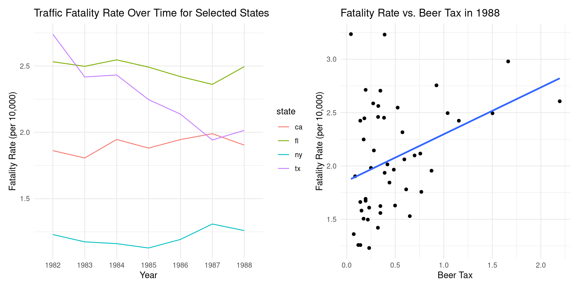
Stock and Watson (1988)
Imagine a government is considering increasing the tax on alcohol to reduce traffic-related deaths. A crucial question for economists is: how can we estimate the causal impact of such a policy?
To answer this, we need to overcome a fundamental challenge: states with higher beer taxes might also have other characteristics that influence traffic fatalities, such as better roads or stricter law enforcement.
- A simple comparison across states at a single point in time might therefore be misleading.
This is where panel data becomes an invaluable tool.
Stock and Watson (1988) (Cont.)
We need two requirements on our data:
Requirement 1: Information Before and After the Policy Change (Time Dimension) We need to observe traffic fatality rates in states before and after any changes in beer taxes. This allows us to see what happens within a state when the policy changes.
Requirement 2: Information from Multiple Entities (Cross-Sectional Dimension) We need data from the same states over consecutive periods. This allows us to compare the changes in fatality rates in states that changed their beer tax to those that did not.
Meekes, Hassink, Kalb (2024)
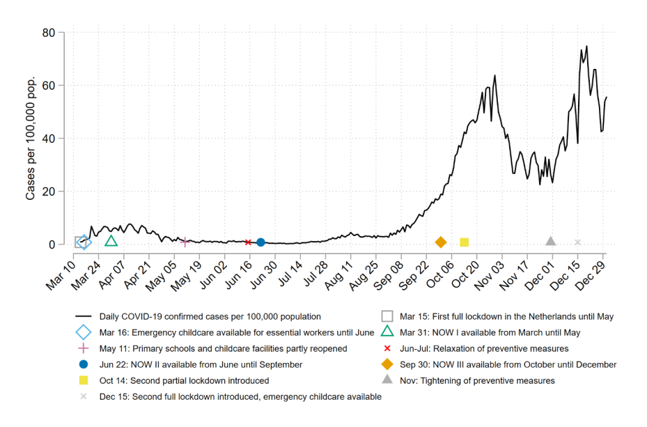
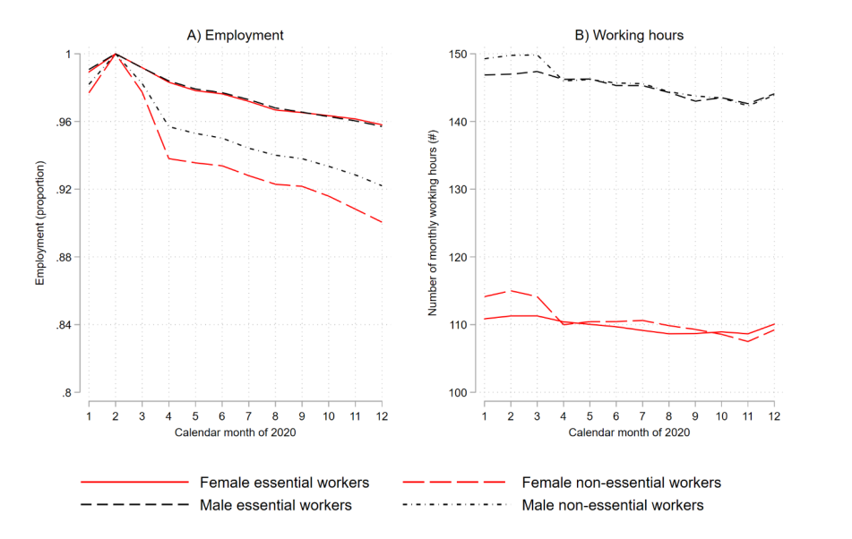
How to estimate the impact of the Covid-outbreak March 2020 on behaviour by individual persons?
The Netherlands: Lockdown from March 16th 2020 onwards.
What data do we need to investigate the impact of the lockdown?
- Requirement 1: We need information from before the lockdown and during the lockdown. Dimension: time
- Requirement 2: We need information from the same persons (or firms) in consecutive periods. Dimension: cross-sectional dimension.
Methodological claim: empirical analyses that are not based on panel data are in general terms not very strong (= the results can easily be falsified).
The two figures below give an impression about what happened in 2020 in the Netherlands.
Meekes, Hassink, Kalb (2024) (Cont.)
Meekes, Hassink, Kalb (2024) (Cont.)
Advantages of Panel Data
Advantages of Panel Data
Examples: Why Panel Data Is Needed?
“Year of Birth” cohorts are followed across time. The research question is “do households sell their house when they become old?” The figure below cannot address this question because from one cross-section to another, it is not possible to disentangle cohort effects from age effects.
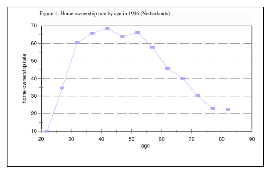
Home Ownership
Examples: Why Panel Data Is Needed?
The figure below is constructed by panel data. The figure indicates strong cohort effects! For each birth cohort, in various years (\(t= 1,2,3,\dots,12\)) the average Dutch home ownership is given.
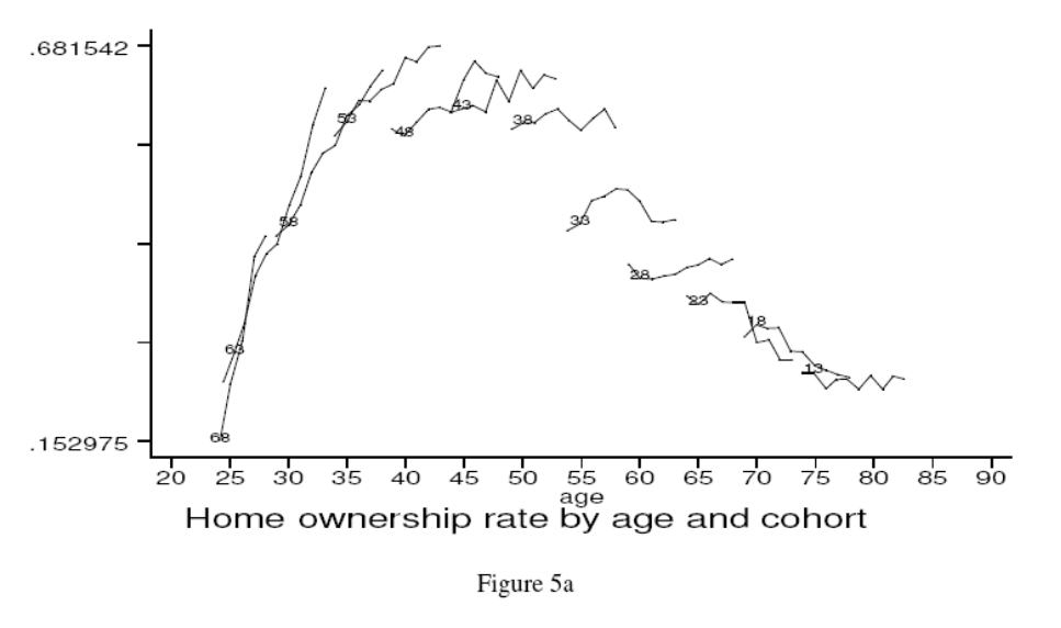
From the cross section it looks like (on average) home ownership rate peaks at around 69%. However, this not necessarily the same for two different cohorts. E.g., compare the 1953 with the 1948 cohort.
Between vs. Within Variation
- Between variation: the cross-sectional variation (across individuals). For example:
| Profit (= dependent variable) | Innovation (=explanatory variable) | |
|---|---|---|
| Firm A | 500 thousand Euros | 1 percent |
| Firm B | 750 thousand Euros | 3 percent |
- Between variation (across firms): as a result of the increased innovation (from 1 percent to 3 percent) the profits increase from 500 thousand Euros to 750 thousand Euros.
Between vs. Within Variation (Cont.)
- Within variation: the time-series variation (for a given individual). So the variation within individuals. For example:
| Profit (= dependent variable) | Innovation (=explanatory variable) | |
|---|---|---|
| Time 1 | 500 thousand Euros | 1 percent |
| Time 2 | 550 thousand Euros | 3 percent |
Within variation (for a given firm): as a result of the increased innovation (from 1 percent to 3 percent (thus by 2 percentage points) the profits increase from 500 thousand Euros to 550 thousand Euros from \(t=1\) to \(t=2\)
Economists are usually interested in the within variation more than in the between variation.
To measure the within variation of x on y, we need to control for individual effects. Consequently, it allows for correlation between the individual effect and the explanatory variable.
Advantages of Panel Data
- Estimation of dynamic models (or transition models) is impossible in the case of a time series of cross sections (panel data).
Example: Why Panel Data is Needed?
Let’s assume that a cross-section study suggests that female labor force participation is equal to 50%. There are two extreme possibilities that we cannot distinguish between cross-sections:
- Possibility 1: 50% of the females are always employed (annual job turnover rate is 0%)
- Possibility 2: In a homogenous population, there is a 50% turnover rate each year.
We need panel data to solve this issue.
Advantages of Panel Data (Cont.)
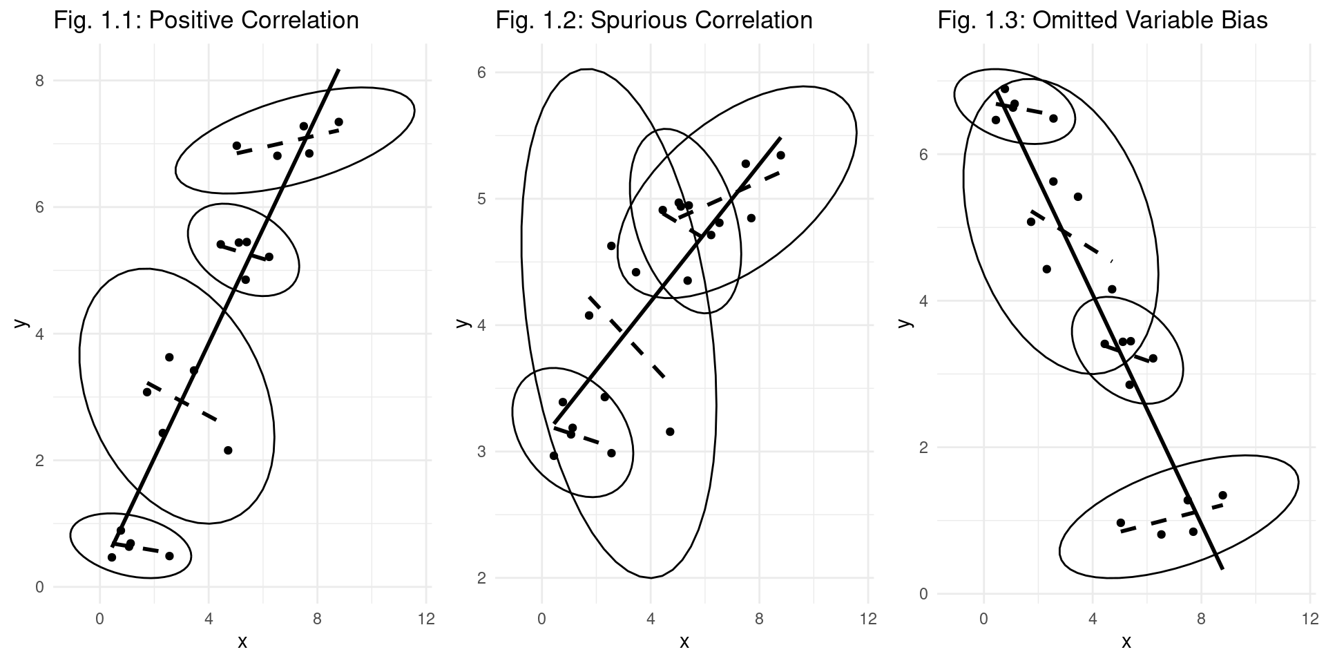
- The primary reason for using panel data is to solve the statistical problem of omitted variables. See the figure below. For each of the N individuals (here three individuals) there is a separate scatter diagram.
- The slope of the solid line is the slope of the regression equation of OLS on all data of all individuals together.
- The slope of the dashed line is the slope of the regression equation in which it is corrected for the individual effect.
- In the figures below, the slope of the dashed lines is different from the slope of the solid line.
Panel Data Structure
Panel Data Models
Specification 1: Cross section: In the first week we considered cross sections:
- A random sample of N firms may have the following regression equation:
\[ \text{Profit} = \beta_0 + \beta_1 \text{Innovation} + \beta_2 \text{Firm Size} + u \]
Cross-sectional dimension \(N\).
- Important: the explanatory variables may be correlated.
- There is one intercept \(\beta_0\). This equation can be reformulated as by adding a subscript \(i\) for the \(i\)-th individual firm:
\[ \text{Profit}_i = \beta_0 + \beta_1 \text{Innovation}_i + \beta_2 \text{Firm Size}_i + u_i \]
Time Series Dimension
Specification 2: Time Series: In the third week we considered the following static time-series model. It is based on a data set containing outcomes for one firm, which is observed over T periods.
\[ \text{Profit}_t = \beta_0 + \beta_1 \text{Innovation}_t + \beta_2 \text{Firm Size}_t + u_t \]
Time dimension \(T\).
Again, there is one intercept \(\beta_0\)
In this equation, we add a subscript \(t\) for the \(t\)-th period:
Panel Data Specification
Specification 3: Panel data is a combination of the previous two equations:
\[ \text{Profit}_{it} = \beta_0 + \beta_1 \text{Innovation}_{it} + \beta_2 \text{Firm Size}_{it} + u_{it} \]
for \(i=1,\dots, N\), \(t=1,\dots, T\).
Again, the only intercept is \(\beta_0\). It has a cross-sectional dimension N and a time dimension T.
- Subscript i refers to individual (firm) and subscript t denotes time.
- Important: the explanatory variables innovation and firm size may be correlated.
Issue 1: Can equation (3) be generalized by N intercepts \(\alpha_i\). Does each firm (subscript \(i\)) have their own intercept?
Panel Data Specification (Cont.)
\[ \text{Profit}_{it} = \alpha_i + \beta_1 \text{Innovation}_{it} + \beta_2 \text{Firm Size}_{it} + u_{it} \]
Issue 2: Is there any correlation between these \(N\) intercepts \(\alpha_i\) and each of the explanatory variables innovation and firm size?
Issue 3: Should variables that remain constant within individual firms be treated differently? E.g. in the following specification, firm size does not change across time. Thus, frmsizeᵢ has no subscript \(t\), in case the size of the firms is constant in all of the \(T\) periods. \[ \text{Profit}_{it} = \beta_0 + \beta_1 \text{Innovation}_{it} + \beta_2 \text{Firm Size}_{i} + u_{it} \]
Issue 4: Are the explanatory variables of the regression equation strictly exogenous? This is an econometric issue that is required for unbiased estimators. It will be explained below further.
Structure of Panel Data
- Imagine tracking the GDP and foreign investment for 3 countries over 4 years.
| Country (i) | Year (t) | GDP (\(y_{it}\)) | Investment (\(X_{it}\)) |
|---|---|---|---|
| USA | 2019 | 21.4 | 0.25 |
| USA | 2020 | 20.9 | 0.16 |
| USA | 2021 | 23.0 | 0.36 |
| USA | 2022 | 25.4 | 0.13 |
| Germany | 2019 | 3.8 | 0.14 |
| Germany | 2020 | 3.8 | 0.13 |
| … | … | … | … |
| Japan | … | … | … |
- Here, \(N=3\) and \(T=4\). In this course, we take \(N\) large and \(T\) relative small.
- The data has both a cross-sectional dimension (comparing USA, Germany, Japan in one year) and a time-series dimension (tracking the USA from 2019-2022).
Balanced vs. Unbalanced Panel Data
- Balanced Panel Data
- Definition: A dataset where each cross-sectional unit (e.g., individual, firm, country) is observed for the exact same number of time periods.
- Structure: If there are ‘N’ units and ‘T’ time periods, the total number of observations is exactly N x T.
- Characteristics:
- No missing observations for any unit over the time span.
- Considered the “ideal” scenario for analysis as it simplifies calculations and avoids issues related to missing data.
- Provides a complete and consistent dataset across all entities and time.
- Unbalanced Panel Data
- Definition: A dataset where at least one cross-sectional unit has missing data for one or more time periods.
- Structure: The total number of observations is less than N x T.
- Characteristics:
- More common in real-world research due to factors like survey attrition, entities entering or leaving the sample (e.g., firm closures), or data collection errors.
- Can still be used for robust analysis, as most modern statistical software can handle unbalanced panels.
The Individual-Specific Effect
Suppose the following “true model”:
\[ y_{it} = a_i + \beta_1x_{1it} + ... + \beta_kx_{kit} + u_{it} \quad i=1,...,N;t=1,...,T \]
Where:
- \(a_i\) is the individual-specific effect (a random variable)
- \(u_{it}\) is the idiosyncratic (i.i.d.: identically and independently distributed) error term with expected value zero and constant variance.
- N: cross-sectional dimension; T: time-dimension
- There are k different explanatory variables.
The Individual-Specifc Effect
The constant \(a_i\) captures all individual-specific variables that are not observed by the researcher; e.g. motivation (it is referred to as unobserved heterogeneity).
It is possible that \(E(a_i | x_{i11},..,x_{i1k},..,x_{iT1},...,x_{iTk}) \neq 0\) (e.g. in an equation where wage is the dependent variable,
motivation(subsumed in \(a_i\)) might be correlated with the RHS-variableexperience).
Strict Exogeneity
- In simple words strict exogeneity means we have:
- No models with a lagged dependent variable
- No models with a feedback mechanism: \(y(t) \leftarrow x(t) \leftarrow y(t-1) \leftarrow x(t-1)\)
Assumption TS.2 (Strict exogeneity)
For each \(t\), the expected value of \(u_t\) given ALL of the \(k\) explanatory variables FOR ALL \(T\) time periods, is equal to zero: \(E[u_t | X] = 0\)
Assumption TS.2 (Contemporaneous exogeneity)
For each t, the expected value of \(u_t\), given ALL of the k explanatory variables in period t, is equal to zero: \(E(u_t | x_{t1},...,x_{tk}) = E(u_t | \mathbf{x}_t) = 0\)
This assumption implies that the error term in period t is uncorrelated with all k regressors in the same period, \(t\): \(Corr(u_t,x_{tj})=0 \quad j=1,...,k\)
Fixed Effects Regression
Fixed Effects
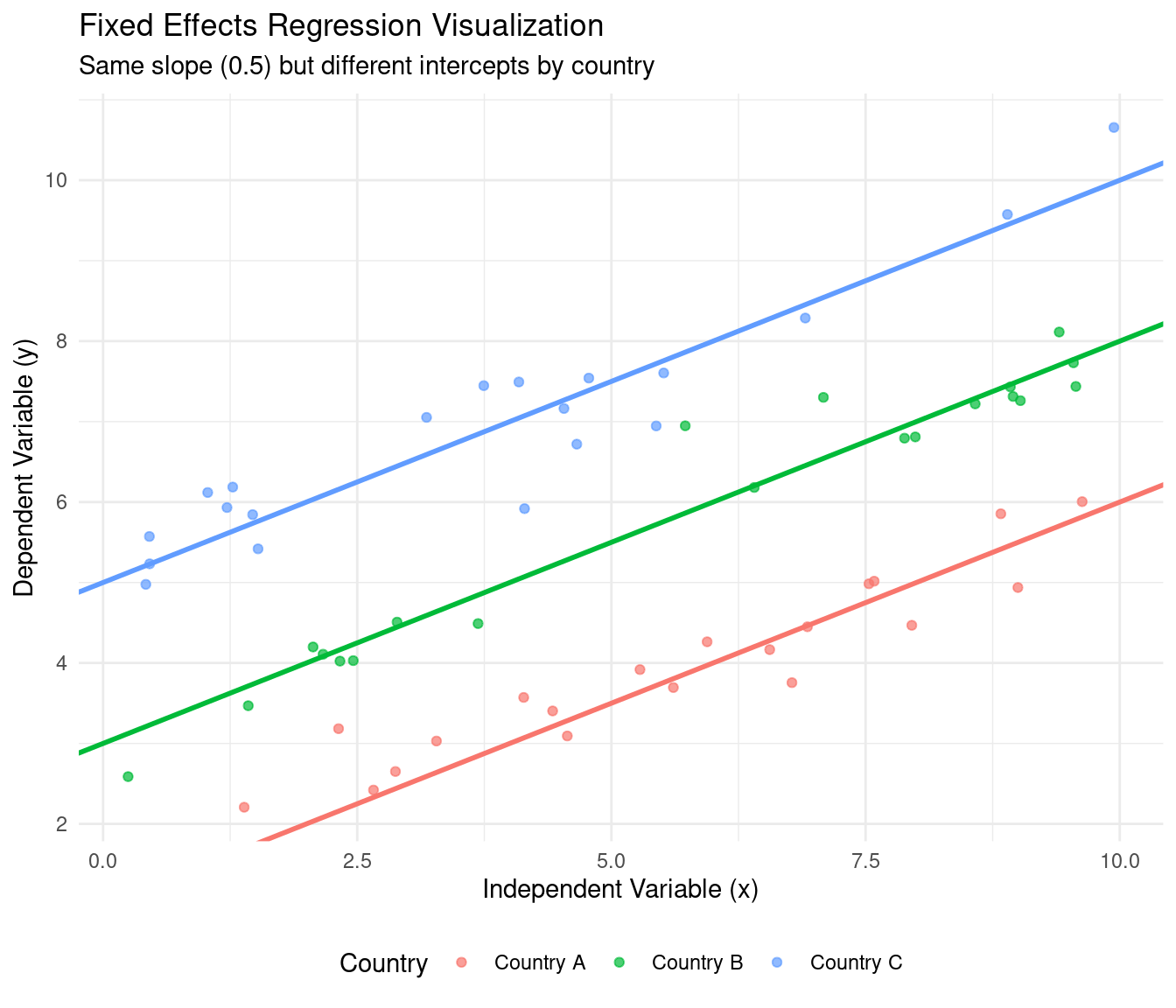
- Core Idea: Treat the individual-specific effects, \(\alpha_i\), as parameters to be estimated. Each individual gets their own intercept.
Definition: Fixed Effects Model
\[ y_{it} = (\beta_0 + \alpha_i) + \beta_1 X_{it} + u_{it} \] or more simply: \[ y_{it} = \alpha_i + \beta_1 X_{it} + u_{it} \] (Here, the \(\alpha_i\) represent the individual-specific intercepts)
- The term “fixed effects” implies that we are making no assumptions about the distribution of the \(\alpha_i\) or their correlation with \(X_{it}\). We allow them to be correlated with the regressors.
The “Within” Estimator for FE
- It is easy to estimate a fixed effects model: it is actually OLS estimation on transformed data
- This fact allows us to estimate the FE model without explicitly estimating \(N\) different intercepts?
- The goal is to eliminate the fixed effect \(\alpha_i\) in \(Y_{it} = \alpha_i + \beta_1 X_{it} + u_{it}\)
Within Transformation
Definition: Within Transformation
Suppose \(y_{it} = \alpha_i + \beta_1 X_{it} + u_{it}\).
Step 1: For each individual \(i\), calculate the time-average of their variables: \[ \bar{y}_i = \frac{1}{T} \sum_{t=1}^{T} y_{it} \quad \text{and} \quad \bar{X}_i = \frac{1}{T} \sum_{t=1}^{T} X_{it} \quad \text{and} \quad \bar{\alpha_i} = \frac{1}{T} \sum_{t=1}^{T} \alpha_i = \alpha_i\]
Step 2: Subtract the individual-specific average from the original model:
\[ \begin{align} y_{it} - \bar{y}_i &= \beta_1 (X_{it} - \bar{X}_i) + (\alpha_i - \bar{\alpha_i}) + (u_{it} + - \bar{u}_i) \\ \ddot{y}_{it} &= \beta_1 \ddot{x}_{it} + \ddot{u}_{it} \end{align} \] The fixed effect \(\alpha_i\) is time-constant, so \(\alpha_i - \bar{\alpha}_i = \alpha_i - \alpha_i = 0\). It drops out!
Step 3: Run OLS on the “de-meaned” data: \[ (y_{it} - \bar{y}_i) = \beta_1 (X_{it} - \bar{X}_i) + (u_{it} - \bar{u}_{it}) \Leftrightarrow \ddot{y}_{it} = \beta_1 \ddot{x}_{it} + \ddot{u}_{it}\] This gives a consistent estimate of \(\beta_1\).
Least Squares Dummy Variable Model
- An alternative, but equivalent, way to get FE estimates is the LSDV model.
LSDV Model
Create a dummy (0/1) variable for each individual \(i\) (except for one, to avoid the dummy variable trap).
Run a single OLS regression including these \(N-1\) dummy variables.
\[ y_{it} = \beta_0 + \beta_1 X_{it} + d_1\alpha_1 + d_2\alpha_2 + ... + d_{N-1}\alpha_{N-1} + u_{it} \]
The estimated coefficient \(\beta_1\) from the LSDV model is identical to the one from the “Within” estimator.
- The coefficients on the dummies (\(\alpha_i\)) are the estimated fixed effects.
- LSDV is impractical for panels with very large \(N\) (e.g., thousands of individuals) due to computational burden. The “Within” estimator is more efficient.
Interpretation of FE Coefficients
Interpretation of Fixed Effects models
In a Fixed Effects model, the coefficient \(\beta_1\) measures:
The average change in \(y\) for a one-unit increase in \(X\) within a given individual over time.
- The FE estimator uses only the variation within each individual (firm/country/etc.) to estimate the coefficients.
- It effectively ignores variation between individuals. You are comparing individual A at time 1 to individual A at time 2, not to individual B.
Time-Constant Variables
- The parameter vector \(\beta\) is identified (‘can be estimated’) due to time-variation in \(x_{it}\) for each individual: the variables differ across time at the level of the individual.
- Individual-specific variables that are constant over time (e.g. gender, year of birth) cannot be included in the model. Their parameters are not identified, as they are incorporated in the individual effect \(a_i\).
Consistency of Fixed Effects
- Why is \(\hat{\beta}_{within}\) a consistent estimator? Let’s assume for simplicity we have a bivariate model: \(y_{it} = x_{it}\beta + a_i + u_{it}\) or
- \(\ddot{y}_{it} = \ddot{x}_{it}\beta + \ddot{u}_{it}\) (5)
- Consistency requires that the error term is uncorrelated with the explanatory variable: \(Corr(\ddot{x}_{it},\ddot{u}_{it}) = Corr(x_{it} - \bar{x}_i, u_{it} - \bar{u}_i) = 0\)
- It means that \(u_{it}\) is uncorrelated with \(\bar{x}_i\)
- It means that \(u_{it}\) is uncorrelated with \(x_{i1},...,x_{iT}\)
- Uncorrelated with x in the past, present and future..
- Conclusion: strict exogeneity is needed (this excludes lagged dependent variables and feedback effects).
- Contemporaneous exogeneity is too weak to prove consistency of the fixed effects estimator \(\beta_{within}\) because it does not exclude correlation between \(u_{it}\) and \(x_{i1},...,x_{iT}\).
Visualization Fixed Effects
Pros and Cons of the Fixed Effects Model
- Pros:
- Controls for all time-invariant omitted variables, whether observed or unobserved. This is its most powerful feature. If you are worried that unobserved
abilityis correlated with botheducation(your X) andwage(your Y), FE solves this problem becauseabilityis constant for an individual. - It is consistent even if the unobserved effect \(\alpha_i\) is correlated with the regressors \(X_{it}\).
- Controls for all time-invariant omitted variables, whether observed or unobserved. This is its most powerful feature. If you are worried that unobserved
- Cons:
- Cannot estimate the effect of time-invariant variables. The “Within” transformation wipes them out.
- For example, you cannot estimate the effect of
genderorraceon wages using a standard FE model, because these variables do not change over time for an individual. - May be less efficient than the Random Effects model if its stricter assumptions hold.
Fixed Effects in Software
Arguably, the fixed effects model is one of the most often-used models in modern econometrics.
Standard statistical software such as
lm()in R orsm.OLS()in Python can implement FE using the LSDV method, but this is often tedious.The
fixest(R) andpyfixest(Python) package provide a very easy way to estimate FE proceding from a dataset that looks like the one on Slide 4.5.This is how that works in practice:
First Differences Estimator
First Differences Estimator
- The regression equation is: \(y_{it} = a_i + \beta_1x_{1it} + ... + \beta_kx_{kit} + u_{it}\)
- Recall that in regression equations the explanatory variables \(x_{it}\) are allowed to be correlated. E.g. education and experience are correlated in a wage equation.
- This is also the case in the fixed effects model. Equation (10) allows for correlation between the explanatory variable \(a_i\) and the other explanatory variables \(x_{1it}, \dots, x_{kit}\).
- Aside from the FE and LSDV estimators, there is another method to estimate parameter \(\beta\) consistently: the first differences estimator.
First Differences: Definition
- Let’s assume there is only one explanatory variable \(x\)
- It is possible to consistently estimate the \(\beta\) parameter by taking first differences
- \(y_{it} = \beta x_{it} + a_i + u_{it}\) (the regression equation in period t)
- \(y_{i,t-1} = \beta x_{i,t-1} + a_i + u_{i,t-1}\) (the regression equation in period t-1)
- The first difference is:
- \(y_{it} – y_{i,t-1} = \beta x_{it} – \beta x_{i,t-1} + a_i – a_i + u_{it} – u_{i,t-1}\), or:
- \(\Delta y_{it} = \beta\Delta x_{it} + \Delta u_{it} \qquad i = 1,...,N; t = 2,...,T\) (11)
- It means that all variables of equation (11) have the same first-differences transformation \(\Delta\)
First Differences: Removal of \(\alpha_i\)
- By taking first differences, the individual effect \(a_i\) is removed from the model.
- We calculate the OLS estimator for equation (11): the so-called first-difference estimator of the regression parameter \(\beta\)
- Denote the first-difference estimator by \(\hat{\beta}_{fdif}\)
- Note that the first period \(t=1\) is used for \(\Delta y_{i2}, \Delta x_{i2}, \Delta u_{i2}\),
Consistency of First Differences
Why is \(\hat{\beta}_{fdif}\) a consistent (or unbiased) estimator? Let’s assume for simplicity we have a bivariate model: \(y_{it} = x_{it}\beta + a_i + u_{it}\) and \(\Delta y_{it} = \Delta x_{it}\beta + \Delta u_{it}\)
Consistency requires that the error term is uncorrelated with the explanatory variable: \(Corr(\Delta u_{it}, \Delta x_{it}) = Corr(u_{it} – u_{i,t-1}, x_{it} – x_{i,t-1}) = 0\)
It means that \(u_{it}\) is uncorrelated with \(x_{i,t-1}, x_{it}, x_{i,t+1}\). In other words, strict exogeneity is needed (no lagged dependent variable, no feedback effects) for consistency (unbiasedness) of the first-difference estimator.
Standard Errors in FD
- In other words, OLS estimation of the FD equation gives the correct standard errors of \(\hat{\beta}_{fdif}\).
- Suppose that there is autocorrelation and heteroskedasticity in \(e_{it}\). In that case \(Var(\hat{\beta}_{fdif})\) is incorrect, because \(\hat{\sigma}_e^2\) is incorrect: robust Newey-West standard errors are necessary.
- Note that it is a different estimator for \(Var(\hat{\beta}_{fdif})\) than the robust standard error (that only corrects for heteroskedasticity)
FE vs. FD
Fixed effects versus First Differences
What do the estimators have in common?
They allow for correlation between \(a_i\) and the explanatory variables \(x_{i1}...x_{iT}\): \(E(a_i | x_{i1},...,x_{iT},...,x_{ki1},...,x_{kiT}) \neq 0\)
The assumption of strict exogeneity (which means that the regression equation contains no feedback mechanism; there is no lag of dependent variable)
Consequence: The parameter estimates of both estimators should be about the same (if the assumption of strict exogeneity is true).
Fixed effects versus First Differences (Cont.)
How do they differ? Assumption about the error term u:
- Fixed effects estimator: \(u_{it}\) is independent over time and across individuals
- First difference estimator (see week 4): \(u_{it} = u_{i,t-1} + e_{it}\)
- \(e_{it}\) is independent over time and across individuals
- Thus \(\Delta u_{it}\) is independent over time and across individuals
- Thus it is assumed that \(u_{it}\) follows a random walk, i.e.: \(u_{it} = u_{i,t-1} + e_{it}\) \(E(e_{it}) = 0\); \(Var(e_{it}) = \sigma_e^2\) (expected value of zero; constant variance)
Consequence: Fixed-effects estimator gives smaller standard errors if the specification is correct and there is strict exogeneity. This estimator is more efficient.
First-difference estimator is preferred if there is a unit root in the error terms: \(u_{it} = u_{i,t-1} + e_{it}\)
Issue: First differences or fixed effects? (II)
If the regression equation is correctly specified,the within estimation procedure and the ‘first-difference estimation’ procedure should yield similar estimates for the parameters \(\beta\).
\(y_{it} = \beta_1x_{1it} +...+ \beta_kx_{kit} + a_i + u_{it}\)
Question: which of the two estimation procedures is preferable?
- Answer: It depends on the time series behavior of \(u_{it}\). If it is a white noise error term, use the within estimation procedure \(\hat{\beta}_{within}\).
- If it follows a random walk (\(u_{it} = u_{i,t-1} + e_{it}\)), use the first-difference procedure \(\hat{\beta}_{fdif}\).
Issue: First Differences or Fixed Effects? (III)
Motivation for the procedure
- Assumption: strict exogeneity (no feedback, no lagged dependent variables).
For ease of exposition here we take one explanatory variable x
Fixed-effects estimator: \(u_{it}\) is identically and independently distributed.
First-difference estimator: \(\Delta u_{it}\) is identically and independently distributed.
- In other words, \(u_{it}\) has a unit root.
Correlation of Error Terms in FD
- The correlation between the error terms of a first-difference estimator is as follows.
Correlation of \(u_{it}\) in the FD model
Assumption: uᵢₜ is identically and independently distributed:
\(Cov(u_{it},u_{is}) = 0\) for \(t \neq s\) (same individual i) \(Cov(u_{it},u_{it}) = \sigma_u^2\) for \(t = s\)
Next, we estimate the model: \(\Delta y_{it} = \Delta x_{it}\beta + \Delta u_{it} \quad i=1,...,N; t = 2,...,T\)
The correlation between \(\Delta u_{it}\) and \(\Delta u_{i,t-1}\) is:
\(Corr(\Delta u_{it}, \Delta u_{i,t-1}) = Corr(u_{it} - u_{i,t-1}, u_{i,t-1} - u_{i,t-2}) = -0.5\).
Hence, the intertemporal correlation of the FD-estimator is -0.5 if \(u_{it}\) is i.i.d.
Motivation for FD Autocorrelation
Correlation of \(u_{it}\) in the FD model
Covariance for the same individual across time:
\[ Cov[aX+bY,cW +dZ]= acCov[X,W]+ adCov[X,Z]+bcCov[Y,W]+bdCov[Y,Z] \]
\[ \begin{align} Cov(u_{it}-u_{i,t-1}, u_{i,t-1}-u_{i,t-2}) &= \\ Cov(u_{it},u_{i,t-1}) &+ Cov(u_{it},-u_{i,t-2}) + Cov(-u_{i,t-1},u_{i,t-1}) + \\ &Cov(-u_{i,t-1},-u_{i,t-2}) \\ &= 0 + 0 - Var(u_{i,t-1}) + 0 \\ &= -\sigma_u^2 \end{align} \]
\[ \begin{align} Var(u_{it} - u_{i,t-1}) &= Var(u_{it}) + Var(-u_{i,t-1}) + 2Cov(u_{it},-u_{i,t-1}) \\ &= \sigma_u^2 + \sigma_u^2 + 0 = 2\sigma_u^2 \end{align} \]
\[ \begin{align} Corr(\Delta u_{it}, \Delta u_{i,t-1}) &= \frac{Cov(\Delta u_{it}, \Delta u_{i,t-1})}{\sqrt{Var(\Delta u_{it}) \cdot Var(\Delta u_{i,t-1})}} \\ &= \frac{-\sigma_u^2}{2\sigma_u^2} = -0.5 \end{align} \]
Fixed Effects or First Differences Procedure
FE vs. FE Procedure
To check for FE versus FD, follow the below procedure:
Step 1: Run a first-difference regression equation of \(\Delta y_{it}\) on \(\Delta x_{it}\)
Step 2: Predict the residuals (which gives \(\Delta \hat{u}_{it}\)) and run a Breusch-Godfrey test for autocorrelation of \(\Delta \hat{u}_{it}\) on \(\Delta \hat{u}_{i,t-1}\) and \(\Delta x_{it}\).
Step 3A: If the estimated coefficient on \(\Delta \hat{u}_{i,t-1}\) is about -0.5 (i.e. -0.5 is within the 95% confidence interval) then there is an indication that \(u_{it}\) is an independent error term (\(u_{it}\) is i.i.d.). Conclusion: prefer within-estimates (fixed effects).
Step 3B: If the estimated coefficient on \(\Delta \hat{u}_{i,t-1}\) is not equal to -0.5 (i.e. -0.5 is outside the 95% confidence interval) then there is an indication that \(u_{it}\) is not an independent error term. Conclusion: prefer first-differences.
If the two procedures yield dramatically different estimates for \(\beta\), the two conclusions are possible, either:
- For some RHS-variables, the assumption of strict exogeneity does not hold.
- The regression model is incorrectly specified. Some important time-varying regressors are missing in the equation.
It is useful to compare the results of both regression procedures.
FD in Software
- In R, the FD model can be estimated using the
plmfunction from theplmlibrary, usingplm(y ~ x1 + x2, data = df, model = "fd"). - In Python, see the implementation below.
- In Stata,
reg d.y d.x, cluster(number)- Some students make the following mistake:
xtreg d.y d.x
- Some students make the following mistake:
Code
# Install the packages if you don't have them already
# install.packages("plm")
# install.packages("AER")

# Load the libraries
library(plm)
library(AER)

# Load the Grunfeld dataset
data("Grunfeld")

# Estimate the first difference model
# We are modeling the change in investment (inv) as a function of
# the change in the value of the firm (value) and the change in capital stock (capital).
fd_model <- plm(inv ~ value + capital, data = Grunfeld, model = "fd")

# Print the summary of the regression results
summary(fd_model)
## Oneway (individual) effect First-Difference Model
##
## Call:
## plm(formula = inv ~ value + capital, data = Grunfeld, model = "fd")
##
## Balanced Panel: n = 10, T = 20, N = 200
## Observations used in estimation: 190
##
## Residuals:
##        Min.     1st Qu.      Median     3rd Qu.        Max.
## -200.889558  -13.889063    0.016677    9.504223  195.634938
##
## Coefficients:
##               Estimate Std. Error t-value  Pr(>|t|)
## (Intercept) -1.8188902  3.5655931 -0.5101    0.6106
## value        0.0897625  0.0083636 10.7325 < 2.2e-16 ***
## capital      0.2917667  0.0537516  5.4281 1.752e-07 ***
## ---
## Signif. codes:  0 '***' 0.001 '**' 0.01 '*' 0.05 '.' 0.1 ' ' 1
##
## Total Sum of Squares:    584410
## Residual Sum of Squares: 345460
## R-Squared:      0.40888
## Adj. R-Squared: 0.40256
## F-statistic: 64.6736 on 2 and 187 DF, p-value: < 2.22e-16
Code
import pandas as pd
import statsmodels.api as sm
from linearmodels.panel import PanelOLS

# Load the Grunfeld dataset
# The statsmodels library includes the Grunfeld dataset
grunfeld_data = sm.datasets.grunfeld.load_pandas().data

# Set firm and year as the index for the panel data model
# The linearmodels package requires a MultiIndex of (entity, time)
grunfeld_data = grunfeld_data.set_index(['firm', 'year'])

# Define the dependent and independent variables
dependent = grunfeld_data['invest']
exog = sm.add_constant(grunfeld_data[['value', 'capital']])

# Estimate the first difference model
# The PanelOLS function with the entity_effects=True argument
# when applied to first-differenced data is equivalent to a first-difference model.
# A more direct way is to difference the data manually.

# 1. Manual First-Differencing
grunfeld_diff = grunfeld_data.groupby('firm').diff().dropna()
dependent_diff = grunfeld_diff['invest']
exog_diff = sm.add_constant(grunfeld_diff[['value', 'capital']])

# We use OLS on the differenced data.
# Note: For a first-difference model, the intercept represents the average time trend.
fd_model_manual = sm.OLS(dependent_diff, exog_diff)
fd_results = fd_model_manual.fit()

# Print the summary of the regression results from our manual first difference
print("First Difference Model Results (Manual Approach)")
## First Difference Model Results (Manual Approach)
print(fd_results.summary())
##                             OLS Regression Results
## ==============================================================================
## Dep. Variable:                 invest   R-squared:                       0.411
## Model:                            OLS   Adj. R-squared:                  0.405
## Method:                 Least Squares   F-statistic:                     71.76
## Date:                Wed, 29 Oct 2025   Prob (F-statistic):           2.25e-24
## Time:                        12:56:40   Log-Likelihood:                -1071.0
## No. Observations:                 209   AIC:                             2148.
## Df Residuals:                     206   BIC:                             2158.
## Df Model:                           2
## Covariance Type:            nonrobust
## ==============================================================================
##                  coef    std err          t      P>|t|      [0.025      0.975]
## ------------------------------------------------------------------------------
## const         -1.6539      3.200     -0.517      0.606      -7.963       4.656
## value          0.0897      0.008     11.271      0.000       0.074       0.105
## capital        0.2906      0.051      5.741      0.000       0.191       0.390
## ==============================================================================
## Omnibus:                       46.816   Durbin-Watson:                   1.611
## Prob(Omnibus):                  0.000   Jarque-Bera (JB):              550.345
## Skew:                           0.348   Prob(JB):                    3.12e-120
## Kurtosis:                      10.919   Cond. No.                         409.
## ==============================================================================
##
## Notes:
## [1] Standard Errors assume that the covariance matrix of the errors is correctly specified.
Code
* 1. Load Stata's built-in Grunfeld dataset
* The 'clear' option removes any data currently in memory
webuse grunfeld, clear

* 2. Declare the data as a panel dataset
* Stata needs to know the panel identifier ('company') and the time variable ('time')
xtset company time

* 3. Estimate the first difference model
* We use the 'xtreg' command with the 'fd' option.
* Note: Stata's Grunfeld dataset uses the variable names mvalue and kstock.
xtreg invest mvalue kstock, fd
What did we do?
- We discussed several issues:
- Motivation for and structure of panel data
- Within variation versus between variation.
- Within effects versus between effects.
- Estimators for within effects: the fixed effects and the first-difference estimator.
- Advantage: we correct for unobserved effects, which are allowed to correlate with the explanatory variables.
- Estimators for between effects: Pooled OLS estimator; Random effects (next lecture)
The End
![]()
Empirical Economics: Lecture 4 - Panel Data I