| Variable | Dim | Mean | SD | Min | Max | Observations |
|---|---|---|---|---|---|---|
| ___________ | _________ | |||||
| union | overall | 0.244 | 0.43 | 0 | 1 | N = 4360 |
| between | 0.329 | 0 | 1 | n = 545 | ||
| within | 0.276 | -0.631 | 1.119 | T = 8 | ||
| ___________ | _________ | |||||
| black | overall | 0.116 | 0.32 | 0 | 1 | N = 4360 |
| between | 0.32 | 0 | 1 | n = 545 | ||
| within | 0 | 0.116 | 0.116 | T = 8 | ||
| ___________ | _________ | |||||
| educ | overall | 11.767 | 1.746 | 3 | 16 | N = 4360 |
| between | 1.748 | 3 | 16 | n = 545 | ||
| within | 0 | 11.767 | 11.767 | T = 8 | ||
| ___________ | _________ | |||||
| hisp | overall | 0.156 | 0.363 | 0 | 1 | N = 4360 |
| between | 0.363 | 0 | 1 | n = 545 | ||
| within | 0 | 0.156 | 0.156 | T = 8 | ||
| ___________ | _________ | |||||
| exper | overall | 6.515 | 2.826 | 0 | 18 | N = 4360 |
| between | 1.655 | 3.5 | 14.5 | n = 545 | ||
| within | 2.292 | 3.015 | 10.015 | T = 8 | ||
| ___________ | _________ | |||||
| expersq | overall | 50.425 | 40.782 | 0 | 324 | N = 4360 |
| between | 26.351 | 17.5 | 215.5 | n = 545 | ||
| within | 31.143 | -44.075 | 158.925 | T = 8 |
Empirical Economics
Lecture 5: Panel Data II
Outline
Course Overview
- Linear Model I
- Linear Model II
- Time Series and Prediction
- Panel Data I
- Panel Data II
- Binary Outcome Data
- Potential Outcomes and Difference-in-differences
- Instrumental Variables
This lecture
Classification of panel data models
Pooled OLS estimator
Random-effects estimator
Random effects or fixed effects: Hausman test
Pooled OLS or Random effects
Line of reasoning with panel data
Material: Wooldridge Chapter 13: 13.1, 13.3, 13.4, 13.5
Motivation
Example: panel information of 900 international businesses (firms). Years: 2019, 2020, 2021.
Variable of interest: Profits of these international firms.
Research question: can we explain the volume of profits by the country of origin (= location of headquarter)?
- E.g., firm has its headquarter in UK, The Netherlands, Germany or France (4 options).
For one year (cross section)? Answer: YES (reference group: Germany)
\[ \text{Profits}_{i} = \beta_{0} + \beta_{1}UK_{i} + \beta_{2}France_{i} + \beta_{3}Netherlands_{i} + u_{i} \]
- for \(i=1,...,900\)
For three years? Answer: It depends.
- This week: various panel methods contrasted.
Motivation (Cont.)
Regression equation is specified as:
\[ \text{Profits}_{it} = a_{i} + \beta_{1}UK_{i} + \beta_{2}France_{i} + \beta_{3}Netherlands_{i} + u_{it} \]
- with \(i = 1,...,900; t = 2019,2020,2021\)
UK, France, Netherlands and Germany are 0-1 indicators:
\[ UK_{i} + France_{i} + Netherlands_{i} + Germany_{i} = 1 \]
Motivation (Cont.)
Can we estimate the regression parameters by the first difference estimator?
- Answer: No, because \(\Delta UK_{i} = 0\), \(\Delta France_{i} = 0\) and \(\Delta Netherlands_{i} = 0\)
\[ \Delta \text{Profits}_{it} = \beta_{1}\Delta UK_{i} + \beta_{2}\Delta France_{i} + \beta_{3}\Delta Netherlands_{i} + \Delta u_{it} \]
Can we estimate the regression parameters with the fixed effects estimator?
- Answer: No, because \(\ddot{UK}_{it} = UK_{it} - \tfrac{1}{T}\sum_{t=1}^Y UK_{it} = 0\)
Can we estimate the parameters by the Pooled OLS estimator?
- Answer: Yes:
\[ \text{Profits}_{it} = \beta_{0} + \beta_{1}UK_{i} + \beta_{2}France_{i} + \beta_{3}Netherlands_{i} + v_{it} \]
with \(v_{it} = a_{i} + u_{it}\), \(i = 1,...,900;t = 2019,2020,2021\)
Three Questions
Question 1: Can we apply alternative estimators, next to the Fixed Effects and the First Difference estimator? This week: Pooled OLS.
Question 2: Can we have a panel data estimator that includes country of headquarter? This week: Random Effects estimator
Question 3: Is there any road map for the preferred estimator?
- Five options: 1. First Difference estimator, 2. LSDV estimator, 3. Fixed Effects Estimator, 4. Pooled OLS, 5. Random Effects estimator.
- Also this week: several testing procedures.
Classification of Panel Models
Static Model: A Classification
Consider the following equation:
\[ y_{it} = a_{i} + \beta_{1}x_{1it} + ... + \beta_{k}x_{kit} + u_{it} \quad i=1,...,N; t=1,...,T \]
It leads to the following two questions:
Question 1: Is there any nonzero correlation between \(a_{i}\) and all of the k RHS vars \(x_{it}\)? Is it nonzero in all T time periods?
- \(E(a_{i} | x_{i11},..,x_{i1k},..,x_{iT1},...,x_{iTk}) = 0\)
- \(E(a_{i} | x_{i11},..,x_{i1k},..,x_{iT1},...,x_{iTk}) \neq 0\)?
Static Model: A Classification (Cont.)
- Question 2: Are all of the k variables \(x_{it}\) strictly exogenous (conditional on the unobserved individual effect \(a_{i}\))?
- \(E(u_{it} | x_{i11},..,x_{i1k},..,x_{iT1},...,x_{iTk}, a_{i}) = 0\) (thus, no lagged dependent variables, no feedback mechanism)
- In all of the estimators of last week we assumed that the exogenous time-varying regressors are strictly exogenous. (conditional on the unobserved effect):
- \(E(u_{it} | x_{i11},..,x_{i1k},..,x_{iT1},...,x_{iTk}, a_{i}) = 0\)
- So again: no lagged dependent variables; no feedback mechanism.
- In explaining estimation procedures, we assume a balanced panel: for every cross-sectional unit, we have the same number of time periods T.
- Model: \(y_{it} = a_{i} + \beta_{1}x_{1it} + ... + \beta_{k}x_{kit} + u_{it} \quad i=1,...,N;t=1,...,T\)
- Software allows for estimation of unbalanced panels, in which not all units have T observations. Thus the i-th individual has \(T_{i}\) observations.
Table A: Estimation Methods
- Estimation methods under different assumptions of strict exogeneity and on the correlation between the individual effect and RHS-variables:
| \(E(a_{i} | X_{i11},..,X_{i1k},..,X_{iT1},..,X_{iTk}) \neq 0\), Correlation between \(a_{i}\) and all of the explanatory variables is allowed to be nonzero | \(E(a_{i} | X_{i11},..,X_{i1k},..,X_{iT1},..,X_{iTk}) = 0\), A zero correlation between \(a_{i}\) and all of the explanatory variables is assumed. | |
|---|---|---|
| All \(x_{it}\) strictly exogenous | 1. First differences 2. LSDV procedure 3. Within estimation |
4. Random effects |
| Some \(x_{it}\) not strictly exogenous | Instrumental Variables (IV) | 5. Pooled OLS (no lagged dependent variables) 6. Instrumental variables (IV) (lagged dep. vars. Included) |
Table B: Estimating Effect of Time-Invariant Variables
| No estimation of \(\gamma\): no effect of \(z_{i}\) on \(y_{it}\) | Estimation of \(\gamma\): effect of \(z_{i}\) on \(y_{it}\) | |
|---|---|---|
| All \(x_{it}\) strictly exogenous | 1. First differences 2. LSDV procedure 3. Within estimation |
4. Random effects |
| Some \(x_{it}\) not strictly exogenous | Instrumental Variables (IV) | 5. Pooled OLS (no lagged dependent variables) 6. Instrumental variables (IV) (lagged dep. vars. Included) |
- The model here is: \(y_{it} = a_{i} + \beta_{1}x_{1it} + ... + \beta_{k}x_{kit} + \gamma_{1}z_{1i} + ... + \gamma_{h}z_{hi} + u_{it}\)
- The variables \(z\) do not change across time but they are different across individuals
- E.g. \(z_{i}\): gender and ethnicity in wage equation
- \(z_{i}\) picks up the between variation (between individuals).
- Between individuals: cross-sectional perspective
- \(x_{it}\) picks up the within variation (within individuals)
- Within individuals: time-series perspective for a given individual
- Economists are usually more interested in within variation.
Pooled OLS
Assumptions
Suppose that instead one estimates the following model by OLS: \[y_{it} = \beta_1x_{1it} + ... + \beta_kx_{kit} + v_{it} \quad i=1,\dots,N;t=1,\dots,T\]
Where \(v_{it} = a_i + u_{it}\) (=individual specific effect + idiosyncratic error term)
In this model, is it assumed that:
\(E(v_{it} | x_{i11},..,x_{i1k},..,x_{iT1},...,x_{iTk}) = 0\) so that, in all \(k\) explanatory variables in all \(T\) time periods:
- \(E(a_i | x_{i11},..,x_{i1k},..,x_{iT1},...,x_{iTk}) = 0\) and
- \(E(u_{it} | x_{i11},..,x_{i1k},..,x_{iT1},...,x_{iTk}, a_i) = 0\)
Violation of this assumption leads to a biased estimate of the regression parameters \(\beta\).
- An application will be given later.
Strict Exogeneity
- In simple words strict exogeneity means we have:
- No models with a lagged dependent variable
- No models with a feedback mechanism: \(y(t) \leftarrow x(t) \leftarrow y(t-1) \leftarrow x(t-1)\)
Assumption TS.2 (Strict exogeneity)
For each \(t\), the expected value of \(u_t\) given ALL of the \(k\) explanatory variables FOR ALL \(T\) time periods, is equal to zero: \(E[u_t | X] = 0\)
Assumption TS.2 (Contemporaneous exogeneity)
For each t, the expected value of \(u_t\), given ALL of the k explanatory variables in period t, is equal to zero: \(E(u_t | x_{t1},...,x_{tk}) = E(u_t | \mathbf{x}_t) = 0\)
This assumption implies that the error term in period t is uncorrelated with all k regressors in the same period, \(t\): \(Corr(u_t,x_{tj})=0 \quad j=1,...,k\)
Violation of Exogeneity
- Violation of the strict exogeneity assumption while assumption contemporaneous exogeneity is satisfied
Example: Dynamic variable with lagged dependent variable
\(y_t = \alpha_0 + \alpha_1y_{t-1} + \delta_1z_t + u_t\)
- \(u_t\) is assumed to be an idiosyncratic error term and contemporaneously exogenous: \(E(u_t | y_{t-1}, z_t) = 0\), so that OLS yields consistent estimates.
- However, \(y_{t-1}\) is NOT a strictly exogenous variable:
- The assumption of strict exogeneity implies that \(u_t\) is uncorrelated not only with \(\mathbf{x}_t = (y_{t-1}, z_t)'\), but also with \(\mathbf{x}_{t+1} = (y_t, z_{t+1})'\)
- According to equation (7), \(y_t\) and \(u_t\) are related to each other. In other words, \(E(u_t | \mathbf{x}_{t+1}) = E(u_t | y_t, z_{t+1}) \neq 0\),
- Thus the lagged dependent variable \(y_{t-1}\) is not strictly exogenous the model.
Violation of Exogeneity Examples
Example: Models with a feedback mechanism
\(gGDP_t = \alpha_0 + \delta_0r_t + u_t\) (8)
- gGDP: GDP-growth rate
- \(r_t\): Interest rate, which is assumed to be contemporaneously exogenous: \(E(u_t | r_t) = 0\)
- The independent variable \(r_t\) depends on the lagged value of the dependent variable (feedback mechanism): \(r_t = \gamma_0 + \gamma_1(gGDP_{t-1} – 3) + v_t\) (9)
- Equation (9) implies that \(r_{t+1}\) depends on \(gGDP_t\) and consequently on \(u_t\).
- \(E(u_t | \mathbf{x}_{t+1}) = E(u_t | r_{t+1}) \neq 0\)
- Thus \(r_t\) is not strictly exogenous in the model.
Pooled OLS Estimator
The Pooled OLS Estimator is an estimator for a zero correlation between \(\alpha_i\) and the explanatory variables
Now we assume that there is no correlation between \(\alpha_i\) and \(x_{it}\)
One of two methods we treat this week:
- Pooled OLS (now)
- Random effects (later)
Pooled OLS Estimation
- Now we assume that there is no correlation between \(a_i\) and all of the \(k\) explanatory variables \(x_{it}\).
- Equation (12) can be estimated with OLS. This is referred to as pooled OLS: \[y_{it} = \beta_1x_{1it} + \dots + \beta_kx_{kit} + v_{it} \quad (12)\]
- For which \(v_{it} = a_i + u_{it}\) where \(u_{it}\) is i.i.d.
- As a result of the identical distribution: \(\text{Var}(v_{it}) = \text{Var}(v_{i,t-1})\)
- In a pooled regression \(v_{it} = a_i + u_{it}\)
- So, in equation (12), it is assumed that: \(E(a_i | x_{i11}, \dots, x_{i1k}, \dots, x_{it1}, \dots, x_{itk}) = 0\) and \(E(u_{it} | x_{i11}, \dots, x_{i1k}, \dots, x_{it1}, \dots, x_{itk}, a_i) = 0\)
- \(a_i\) is uncorrelated with all of the explanatory variables.
- \(u_{it}\) is uncorrelated with all of the explanatory variables and \(a_i\).
Autocorrelation in Pooled OLS
The autocorrelation between the error terms \(v_{it}\) and \(v_{i,t-1}\) of equation (12) is:
\[ \text{Corr}(v_{it}, v_{i,t-1}) = \frac{\text{Cov}(v_{it}, v_{i,t-1})}{\sqrt{\text{Var}(v_{it})\text{Var}(v_{i,t-1})}} = \frac{\text{Cov}(v_{it}, v_{i,t-1})}{\text{Var}(v_{it})} \]
We can show that the numerator is:
\[ \begin{align*} \text{Cov}(v_{it}, v_{i,t-1}) &= \text{Cov}(a_i + u_{it}, a_i + u_{i,t-1}) \\ &= \text{Cov}(a_i, a_i) + \text{Cov}(a_i, u_{i,t-1}) + \text{Cov}(u_{it}, a_i) + \text{Cov}(u_{it}, u_{i,t-1}) \\ &= \sigma_a^2 \quad (=0) \quad (=0) \quad (=0) \\ &= \text{Var}(a_i) + 0 + 0 + 0 \\ &= \sigma_a^2 \end{align*} \]
Autocorrelation in Pooled OLS (Cont.)
And the denominator is: \[ \begin{align*} \text{Var}(v_{it}) &= \text{Var}(a_i + u_{it}) \\ &= \text{Var}(a_i) + \text{Var}(u_{it}) + 2\text{Cov}(a_i, u_{it}) \\ &= \sigma_a^2 + \sigma_u^2 \quad (=0) \\ &= \sigma_a^2 + \sigma_u^2 \end{align*} \]
So that:
\[ \frac{\text{Cov}(v_{it}, v_{i,t-1})}{\text{Var}(v_{it})} = \frac{\sigma_a^2}{\sigma_a^2 + \sigma_u^2} \]
Conclusion: In pooled OLS there is always autocorrelation.
- The estimation procedure for Pooled OLS: OLS on with Newey-West robust standard errors, which are similar to clustered standard errors. It corrects for both heteroskedasticity and autocorrelation.
Example: Pooled OLS
- Example: Vella and Verbeek (1998) ask whether unions raise wages.
- They have a panel dataset with individual wages, union membership, and various control variables, of which some are time-varying (e.g. experience), and some are constant over time (e.g. race).
- Estimation procedure:
- We start with the pooled OLS estimator.
- Next, we check for autocorrelation, using the Breusch Godfrey test.
- The parameter on the lagged residual is statistically different from zero (F-value: 27.90).
- We re-estimated the model with the pooled OLS estimator, using clustered standard errors.
Example: Pooled OLS (Cont.)
- This is what the data look like:
Example: Pooled OLS (Cont.)
- Results show that unions raise wages by about 18%
| Pooled OLS | Pooled OLS, Clustered SE | |
|---|---|---|
| * p < 0.1, *** p < 0.1, ** p < 0.05 | ||
| (Intercept) | -0.035 | -0.035 |
| (0.065) | (0.120) | |
| union | 0.180** | 0.180** |
| (0.017) | (0.028) | |
| educ | 0.099** | 0.099** |
| (0.005) | (0.009) | |
| black | -0.144** | -0.144** |
| (0.024) | (0.050) | |
| hisp | 0.016 | 0.016 |
| (0.021) | (0.039) | |
| exper | 0.089** | 0.089** |
| (0.010) | (0.012) | |
| expersq | -0.003** | -0.003** |
| (0.001) | (0.001) | |
| married | 0.108** | 0.108** |
| (0.016) | (0.026) | |
| R2 | 0.187 | 0.187 |
| Num.Obs. | 4360 | 4360 |
Example: Pooled OLS (Cont.)
- Since there is strong evidence for autocorrelation according to the BG-test, cluster standard errors by individual.
| Breusch-Godfrey Test | |
|---|---|
| * p < 0.1, *** p < 0.1, ** p < 0.05 | |
| (Intercept) | -0.025 |
| (0.056) | |
| uhat_lag1 | 0.503** |
| (0.013) | |
| union | -0.028*** |
| (0.015) | |
| educ | 0.001 |
| (0.004) | |
| black | -0.002 |
| (0.020) | |
| hisp | 0.002 |
| (0.018) | |
| exper | 0.004 |
| (0.009) | |
| expersq | -0.000 |
| (0.001) | |
| married | -0.005 |
| (0.014) | |
| R2 | 0.252 |
| Num.Obs. | 4359 |
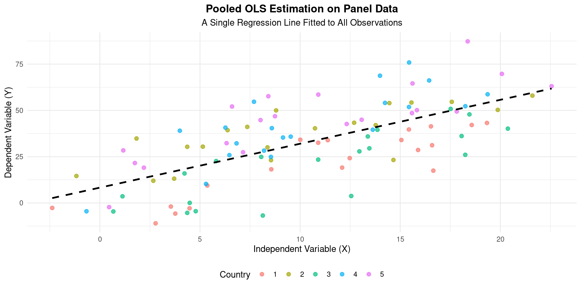
Pooled OLS Visualization
Random Effects
Random Effects Model
Consider the static model:
\[ y_{it} = \beta_1x_{1it} + \dots + \beta_kx_{kit} + a_i + u_{it} \quad (6) \]
for \(i=1,...,N; t=1,...,T\)
The equation (6) does not allow correlation between \(a_i\) and all of the right hand side variables \(x_{1it},...,x_{kit}\) (over all \(T\) periods) \[ E(a_i | x_{1i1},...,x_{1iT},...,x_{ki1},...,x_{kiT}) = 0 \]
The exogenous time-varying regressors are assumed to be strictly exogenous (conditional on the unobserved effect): \[ E(u_{it} | x_{1i1},...,x_{1iT},...,x_{ki1},...,x_{kiT}, a_i) = 0 \]
In simple words: there are neither lagged dependent variables nor is there any feedback mechanism
Random Effects Model (Cont.)
The following is assumed about \(u_{it}\):
- \(E(u_{it}) = 0\); \(\text{Var}(u_{it}) = \sigma_u^2\) (expected value of zero; constant variance)
- \(u_{it}\) is independent over time and across individuals
The following is assumed about \(a_i\):
- \(E(a_i) = 0\); \(\text{Var}(a_i) = \sigma_a^2\) (expected value of zero; constant variance)
- \(a_i\) is independent over time and across individuals
Equation (6) can be rewritten as follows: Model: \(y_{it} = \beta_1x_{1it} + \dots + \beta_kx_{kit} + v_{it} \quad (6)\) \(i=1,...,N; t=1,...,T\) where \[v_{it} = a_i + u_{it} \quad (7)\]
The random effects estimator works as follows. We estimate equation (6), in which the error structure of equation (7) is taken into account.
Correlation Structure Error Terms
- Error term (see slide above): \(v_{it} = a_i + u_{it}\)
- Covariance across two individuals \(i\) and \(j\):
- \(\text{Cov}(v_{it}, v_{jt}) = 0\) for \(i \neq j\)
- \(\text{Cov}(v_{it}, v_{js}) = 0\) for \(i \neq j; t \neq s\)
- Covariance for the same individual across time:
- \(\text{Cov}(aX+bY, cW+dZ) = ac\text{Cov}(X,W) + ad\text{Cov}(X,Z) + bc\text{Cov}(Y,W) + bd\text{Cov}(Y,Z)\)
- So that: \[ \begin{align*} \text{Cov}(v_{it}, v_{is}) &= \text{Cov}(a_i + u_{it}, a_i + u_{is}) \\ &= \text{Cov}(a_i, a_i) + \text{Cov}(a_i, u_{is}) + \text{Cov}(u_{it}, a_i) + \text{Cov}(u_{it}, u_{is}) \\ &= \sigma_a^2 + 0 + 0 + 0 \\ &= \sigma_a^2 \end{align*} \]
Correlation Structure Error Terms
- Variance for an individual: \[\text{Var}(X+Y) = \text{Var}(X) + \text{Var}(Y) + 2\text{Cov}(X,Y)\] \[ \begin{align*} \text{Var}(v_{it}) &= \text{Var}(a_i + u_{it}) \\ &= \text{Var}(a_i) + \text{Var}(u_{it}) + 2\text{Cov}(a_i, u_{it}) \\ &= \sigma_a^2 + \sigma_u^2 + 0 \end{align*} \]
- Thus: \[\text{Corr}(v_{it}, v_{is}) = \frac{\text{Cov}(v_{it}, v_{is})}{\sqrt{\text{Var}(v_{it})\text{Var}(v_{is})}} = \frac{\sigma_a^2}{\sigma_a^2 + \sigma_u^2}\]
- Conclusion: random effects estimator \(\beta_{re}\) takes account of the autocorrelation structure
Random Effects: Further Remarks
Both random effects and pooled OLS allow for the inclusion of time-invariant individual variables (e.g. gender in a wage equation):
\[ y_{it} = a_i + \beta_1x_{1it} + \dots + \beta_kx_{kit} + \gamma_1z_{1i} + \dots + \gamma_rz_{ri} + u_{it} \]
For \(i=1,...,N; \quad t=1,...,T\).
And \(z\) is a vector of individual-specific regressors.
Remember: the effect of \(z\) on \(y\) cannot be estimated (‘is not identified’) in the fixed-effects specification.
Estimation of RE Models (GLS)
- Estimating the RE model can “almost” be done using Pooled OLS.
- If we run Pooled OLS on the data, assuming the RE model, the estimates of \(\beta\) will be unbiased (if the key assumption holds), but they will be inefficient.
- The composite error term \(u_{it} = \alpha_i + \nu_{it}\) creates serial correlation within each individual.
- Solution: Generalized Least Squares (GLS).
- GLS is a method that transforms the data to account for this specific error structure, producing efficient estimates.
- In practice, we use Feasible GLS (FGLS) because we have to estimate the components of the error correlation first. This is what statistical software does automatically.
Interpretation of RE Coefficients
- The RE estimator uses a weighted average of the “within” and “between” variation in the data.
Interpretation of RE Estimates
The coefficient \(\beta_1\) from an RE model is interpreted as:
The estimated change in \(y\) for a one-unit increase in \(x\), assuming the unobserved individual effects \(\alpha_i\) are uncorrelated with \(x\).
- It’s a more general interpretation than in the FE model.
- The reliability of this interpretation hinges entirely on the key RE assumption holding true.
Pros and Cons of the Random Effects Model
- Pros:
- Can estimate the effects of time-invariant variables (e.g., gender, race, industry), because it does not wipe them out.
- More efficient (i.e., has smaller standard errors) than the FE model, if the key assumption (\(E(\alpha_i | X_{it}) = 0\)) is met. It uses both “within” and “between” variation.
- Cons:
- Estimates are biased and inconsistent if the key assumption is violated. This is the critical weakness. If the unobserved effects are correlated with your regressors, the RE model suffers from omitted variable bias.
Hausman Test
RE or FE?
Model: \(y_{it} = \beta_1x_{1it} + \dots + \beta_kx_{kit} + a_i + u_{it} \quad (8)\)
- \(E(a_i | x_{1i1},\dots,x_{1iT},\dots,x_{ki1},\dots,x_{kiT}) = 0\)
- \(E(u_{it} | x_{1i1},\dots,x_{1iT},\dots,x_{ki1},\dots,x_{kiT}, a_i) = 0\)
\(x_{it}\) is strictly exogenous (in simple words: no lagged dependent variables; no feedback mechanism).
Estimation method: Random effects
- Equation (8) can be estimated with random effects, which requires the assumption \(E(a_i | x_{1i1},\dots,x_{1iT},\dots,x_{ki1},\dots,x_{kiT}) = 0\)
- \(\hat{\beta}_{re}\) is a consistent estimator of \(\beta\)
Estimation method: Fixed effects
- Equation (8) can be estimated with fixed effects, which does NOT assume that \(E(a_i | x_{1i1},\dots,x_{1iT},\dots,x_{ki1},\dots,x_{kiT}) = 0\)
- \(\hat{\beta}_{within}\) is a consistent estimator of \(\beta\)
- \(\hat{\beta}_{within}\) is less efficient than \(\hat{\beta}_{re}\): It means that \(\text{Var}(\hat{\beta}_{re}) < \text{Var}(\hat{\beta}_{within})\)
Consequently, random effects yields significant t-statistics more easily than fixed effects.
Comparing FE and RE: The Hausman Test
So which model should we use? FE or RE? The Hausman Test helps us decide.
Intuition:
- The FE estimator is always consistent, whether the unobserved effects \(\alpha_i\) are correlated with \(X\) or not.
- The RE estimator is consistent AND efficient if \(\alpha_i\) and \(X\) are uncorrelated, but inconsistent if they are correlated.
The Test: We compare the coefficient estimates from FE and RE.
- If the coefficients are “close” to each other, it suggests the RE assumption holds, and we should use the more efficient RE model.
- If the coefficients are “far apart” and statistically different, it suggests the RE assumption is violated. We must use the consistent FE model.
Hausman Test Structure
Model: \(y_{it} = \beta_{1}x_{1it} + ... + \beta_{k}x_{kit} + a_{i} + u_{it}\)
\(E(a_{i} | x_{1i1},...,x_{1iT},...,x_{ki1},...,x_{kiT}) = 0\)
\(E(u_{it} | x_{1i1},...,x_{1iT},...,x_{ki1},...,x_{kiT}, a_{i}) = 0\)
Structure:
- Null hypothesis: \(H_{0}: E(a_{i} | x_{1i1},...,x_{1iT},...,x_{ki1},...,x_{kiT}) = 0\)
- Alternative hypothesis: \(H_{1}: E(a_{i} | x_{1i1},...,x_{1iT},...,x_{ki1},...,x_{kiT}) \neq 0\)
Under the null hypothesis (\(H_{0}\)), random effects is preferred (because of the zero correlation between the \(a_{i}\) and the explanatory variables).
- The model can be estimated by random effects and fixed effects.
- If \(H_{0}\) is true, both estimators are unbiased (consistent). However, random effects yields smaller standard errors, so that it is preferred to fixed effects.
If alternative hypothesis (\(H_{1}\)) is true: fixed effects is preferred, because random effects estimator is biased.
Hausman Test Statistic
The test is based on the difference between the coefficient vectors from the two models: \((\hat{\beta}_{FE} - \hat{\beta}_{RE})\).
The Hausman statistic, \(H\), is a measure of the squared distance between the two vectors of coefficients, weighted by the precision (1/variance) of this difference.
- It is constructed so that large, systematic differences between the coefficients lead to a large test statistic.
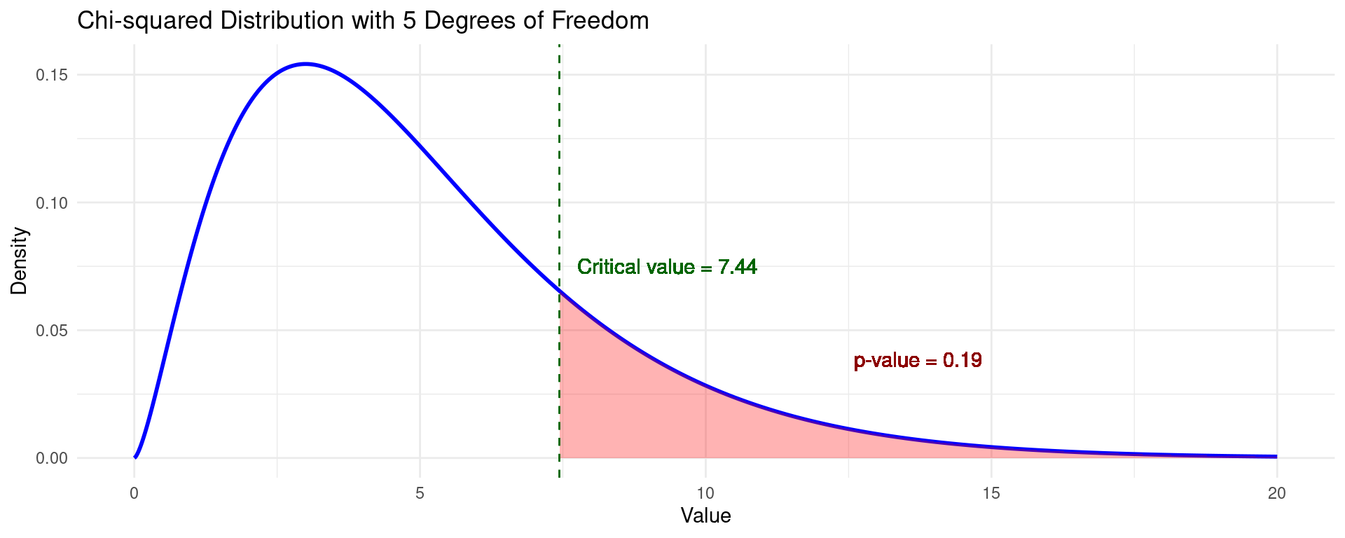
Under the null hypothesis (\(H_0\)), the test statistic follows a Chi-squared distribution with \(k\) degrees of freedom, where \(k\) is the number of time-varying regressors in the model.
\[ H \sim \chi^2(k) \]
\(\chi^2\) Test Visualization
- The \(\chi^2\) distribution is one-sided.
- A significance level \(\alpha\) gives you a critical value on the basis of which a test can be rejected.
- Alternatively, the \(p\)-value can be calculated according to the cdf.
The Hausman Test: Application
Hausman Test: Procedure
\(H_0\): The Random Effects model is the appropriate model. (The difference in coefficients between FE and RE is not systematic, i.e., \(E(\alpha_i | X_{it}) = 0\)).
\(H_A\): The Fixed Effects model is the appropriate model. (The difference in coefficients is systematic, i.e., \(E(\alpha_i | X_{it}) \neq 0\)).
Statistical software calculates a test statistic (Chi-squared) and a p-value.
- If p-value < 0.05 (or your chosen significance level): Reject the null hypothesis. The models are significantly different. Conclude that the RE assumption is likely violated. Use the Fixed Effects model.
- If p-value >= 0.05: Fail to reject the null hypothesis. You do not have evidence that the RE assumption is violated. Use the more efficient Random Effects model.
Example: FE vs. RE
- We use the same dataset as before (Vella and Verbeek, 1998)
- We estimate the model: \(\log \text{Wage} = \alpha_i + \beta_1 \text{Union}_{it} + \beta_2 \text{Exper}_{it} + \beta_3 \text{Exper}^2_{it} + u_{it}\) by FE and RE
- The Hausman test can only compare models with the same variables, hence we only include time-varying control variables.
- The results are shown below:
| FE | RE | |
|---|---|---|
| * p < 0.1, *** p < 0.1, ** p < 0.05 | ||
| union | 0.083** | 0.102** |
| (0.019) | (0.018) | |
| exper | 0.122** | 0.126** |
| (0.008) | (0.008) | |
| expersq | -0.004** | -0.005** |
| (0.001) | (0.001) | |
| (Intercept) | 1.060** | |
| (0.031) | ||
| R2 | 0.177 | 0.151 |
| Num.Obs. | 4360 | 4360 |
Example: Hausman Test
- According to these models, union membership raises wages with 8.3% (FE) or 10.2% (RE).
- The Hausman test clearly rejects the null hypothesis of \(E(\alpha_i | X_{it}) = 0\).
- This implies the fixed effects model is preferable to the random effects model.
    Hausman Test

data:  formula
chisq = 139.94, df = 3, p-value < 2.2e-16
alternative hypothesis: one model is inconsistent
Pooled OLS vs. Random Effects
Pooled OLS vs. RE
To formally decide between Pooled OLS and Random Effects, you should use the Breusch-Godfrey test for random effects.
Purpose of the Test: This test checks whether the variance of the individual-specific effect (\(a_i\)) is equal to zero.
Hypotheses:
- Null Hypothesis (\(H_0\)): \(Var(a_i) = \sigma_a^2 = 0\). There are no significant individual-specific effects. The Pooled OLS model is adequate.
- Alternative Hypothesis (\(H_1\)): \(Var(a_i) = \sigma_a^2 > 0\). There are significant individual-specific effects. The Random Effects model is preferred over Pooled OLS.
Decision Rule:
- If the p-value is high (e.g., > 0.05), you fail to reject the null hypothesis. This suggests that the individual effects are not significant, and you can use the simpler Pooled OLS model.
- If the p-value is low (e.g., < 0.05), you reject the null hypothesis. This provides strong evidence for the presence of individual-specific effects, making the Random Effects model the better choice.
Example: Pooled OLS vs. RE
- Using again the same dataset (Vella and Verbeek, 1998)
- We can now use the full set of control variables.
- The results are shown below.
| Pooled OLS | Random Effects | |
|---|---|---|
| * p < 0.1, *** p < 0.1, ** p < 0.05 | ||
| (Intercept) | -0.035 | -0.107 |
| (0.065) | (0.111) | |
| union | 0.180** | 0.107** |
| (0.017) | (0.018) | |
| educ | 0.099** | 0.101** |
| (0.005) | (0.009) | |
| black | -0.144** | -0.144** |
| (0.024) | (0.048) | |
| hisp | 0.016 | 0.020 |
| (0.021) | (0.043) | |
| exper | 0.089** | 0.112** |
| (0.010) | (0.008) | |
| expersq | -0.003** | -0.004** |
| (0.001) | (0.001) | |
| married | 0.108** | 0.063** |
| (0.016) | (0.017) | |
| R2 | 0.187 | 0.178 |
| Num.Obs. | 4360 | 4360 |
Example: Pooled OLS vs. RE (Cont.)
- The results of the Breusch-Godfrey test show the variance of the unobserved effects \(\text{Var}(\sigma^2_{a}) > 0\).
- This implies the Random Effects model is more reliable.
- Hence the Random Effects model should be preferred.
| Breusch-Godfrey Test | |
|---|---|
| * p < 0.1, *** p < 0.1, ** p < 0.05 | |
| (Intercept) | -0.025 |
| (0.056) | |
| uhat_lag1 | 0.503** |
| (0.013) | |
| union | -0.028*** |
| (0.015) | |
| educ | 0.001 |
| (0.004) | |
| black | -0.002 |
| (0.020) | |
| hisp | 0.002 |
| (0.018) | |
| exper | 0.004 |
| (0.009) | |
| expersq | -0.000 |
| (0.001) | |
| married | -0.005 |
| (0.014) | |
| R2 | 0.252 |
| Num.Obs. | 4359 |
Choosing Panel Models
Reasoning with Panel Data
Line of Reasoning with Panel Data
- Step 1a: Apply pooled OLS \[y_{it} = \beta_1x_{1it} + \dots + \beta_kx_{kit} + v_{it}\]
- Step 1b: Test for autocorrelation of error term with Breusch-Godfrey. Estimated parameter on lagged \(v_{it}\) is \[\text{Corr}(v_{it}, v_{is}) = \frac{\sigma_a^2}{\sigma_a^2 + \sigma_u^2}\]
- Step 1c: Re-estimate pooled OLS with clustered standard errors
- Step 2a: Apply first-differences estimator (FD): \[\Delta y_{it} = \beta_1\Delta x_{1it} + \dots + \beta_k\Delta x_{kit} + \Delta u_{it}\]
- Step 2b: Compute autocorrelation: is the parameter on \(\Delta u_{i,t-1}\) of Breusch-Godfrey equal to -0.5?
- Step 2c: Re-estimate FD with clustered standard errors
- (Continued on next slide.)
Reasoning with Panel Data (Cont.)
Line of Reasoning with Panel Data
- Step 3a: Apply LSDV/ fixed-effects estimator (FE): \[\ddot{y}_{it} = \beta_1\ddot{x}_{1it} + \dots + \beta_k\ddot{x}_{kit} + \ddot{u}_{it}\]
- Step 3b: Compute autocorrelation
- Step 3c: Compare the outcome of the FD estimator with the outcome of the FE estimator
- Step 4a: Apply random effects estimator (RE)
- Step 4b: Test for autocorrelation
- Step 4c: Compare the outcome of the Random effects estimator and Pooled OLS estimator
- Step 5: Test for Random effects versus fixed effects using the Hausman test.
Example (Entire Procedure)
- We apply the five steps on the Vella and Verbeek (1998) dataset
- Step 1a: Apply Pooled OLS:
| Pooled OLS | |
|---|---|
| * p < 0.1, *** p < 0.1, ** p < 0.05 | |
| (Intercept) | -0.035 |
| (0.065) | |
| union | 0.180** |
| (0.017) | |
| educ | 0.099** |
| (0.005) | |
| black | -0.144** |
| (0.024) | |
| hisp | 0.016 |
| (0.021) | |
| exper | 0.089** |
| (0.010) | |
| expersq | -0.003** |
| (0.001) | |
| married | 0.108** |
| (0.016) | |
| R2 | 0.187 |
| Num.Obs. | 4360 |
Example (Entire Procedure) (Cont.)
- Step 1b: Test for autocorrelation of error term with Breusch-Godfrey.
| Breusch-Godfrey Test | |
|---|---|
| * p < 0.1, *** p < 0.1, ** p < 0.05 | |
| (Intercept) | -0.025 |
| (0.056) | |
| uhat_lag1 | 0.503** |
| (0.013) | |
| union | -0.028*** |
| (0.015) | |
| educ | 0.001 |
| (0.004) | |
| black | -0.002 |
| (0.020) | |
| hisp | 0.002 |
| (0.018) | |
| exper | 0.004 |
| (0.009) | |
| expersq | -0.000 |
| (0.001) | |
| married | -0.005 |
| (0.014) | |
| R2 | 0.252 |
| Num.Obs. | 4359 |
Example (Entire Procedure) (Cont.)
- Step 1c: Re-estimate pooled OLS with clustered standard errors
| Pooled OLS, Clustered SE | |
|---|---|
| * p < 0.1, *** p < 0.1, ** p < 0.05 | |
| (Intercept) | -0.035 |
| (0.120) | |
| union | 0.180** |
| (0.028) | |
| educ | 0.099** |
| (0.009) | |
| black | -0.144** |
| (0.050) | |
| hisp | 0.016 |
| (0.039) | |
| exper | 0.089** |
| (0.012) | |
| expersq | -0.003** |
| (0.001) | |
| married | 0.108** |
| (0.026) | |
| R2 | 0.187 |
| Num.Obs. | 4360 |
Example (Entire Procedure) (Cont.)
- Step 2a: Apply first-differences estimator (FD)
- Only time-varying variables remain in the equation.
| FD | |
|---|---|
| * p < 0.1, *** p < 0.1, ** p < 0.05 | |
| (Intercept) | 0.116** |
| (0.020) | |
| union | 0.043** |
| (0.020) | |
| expersq | -0.004** |
| (0.001) | |
| married | 0.038*** |
| (0.023) | |
| R2 | 0.004 |
| Num.Obs. | 3815 |
Example (Entire Procedure) (Cont.)
- Step 2b: Compute autocorrelation: is the parameter on \(\Delta u_{it-1}\) of Breusch-Godfrey equal to -0.5?
- \(-0.5\) is not in the confidence interval. Therefore we prefer FD over the FE estimator (see previous lecture).
| Breusch-Godfrey Test | |
|---|---|
| * p < 0.1, *** p < 0.1, ** p < 0.05 | |
| (Intercept) | 0.005 |
| (0.018) | |
| uhat_lag1 | -0.361** |
| (0.015) | |
| union | 0.020 |
| (0.018) | |
| expersq | -0.000 |
| (0.001) | |
| married | 0.006 |
| (0.021) | |
| R2 | 0.130 |
| Num.Obs. | 3814 |
Example (Entire Procedure) (Cont.)
- Step 2c: Re-estimate FD with clustered standard errors
| FD, Clustered SE | |
|---|---|
| * p < 0.1, *** p < 0.1, ** p < 0.05 | |
| (Intercept) | 0.116** |
| (0.014) | |
| union | 0.043*** |
| (0.022) | |
| expersq | -0.004** |
| (0.001) | |
| married | 0.038 |
| (0.024) | |
| R2 | 0.004 |
| Num.Obs. | 3815 |
Example (Entire Procedure) (Cont.)
- Step 3a: Apply LSDV/fixed-effects estimator (FE)
| FE | |
|---|---|
| * p < 0.1, *** p < 0.1, ** p < 0.05 | |
| union | 0.082** |
| (0.019) | |
| exper | 0.117** |
| (0.008) | |
| expersq | -0.004** |
| (0.001) | |
| married | 0.045** |
| (0.018) | |
| R2 | 0.620 |
| Num.Obs. | 4360 |
Example (Entire Procedure) (Cont.)
- Step 4a: Apply random effects estimator
| Random Effects | |
|---|---|
| * p < 0.1, *** p < 0.1, ** p < 0.05 | |
| (Intercept) | -0.107 |
| (0.111) | |
| union | 0.107** |
| (0.018) | |
| educ | 0.101** |
| (0.009) | |
| black | -0.144** |
| (0.048) | |
| hisp | 0.020 |
| (0.043) | |
| exper | 0.112** |
| (0.008) | |
| expersq | -0.004** |
| (0.001) | |
| married | 0.063** |
| (0.017) | |
| R2 | 0.178 |
| Num.Obs. | 4360 |
Example (Entire Procedure) (Cont.)
- Step 5: Test for Random effects versus fixed effects using Hausman test.
- The Hausman test convincingly rejects the null hypothesis, hence Fixed Effects is preferred over Random Effects.
    Hausman Test

data:  formula
chisq = 31.451, df = 4, p-value = 2.476e-06
alternative hypothesis: one model is inconsistent
Conclusion
Conclusion
This lecture expanded our toolkit for panel data by introducing Pooled OLS and the Random Effects (RE) estimator, providing alternatives to the Fixed Effects (FE) and First Differences models.
The critical choice between Fixed Effects (FE) and Random Effects (RE) hinges on a key assumption: Is the unobserved individual effect (\(a_i\)) correlated with the explanatory variables (\(X_{it}\))?
Model Summary:
- Use Fixed Effects (FE) if you believe \(a_i\) and \(X_{it}\) are correlated. This provides consistent estimates, but you cannot estimate the effect of time-invariant variables.
- Use Random Effects (RE) if you can assume \(a_i\) and \(X_{it}\) are uncorrelated. This model is more efficient (has smaller standard errors) and, importantly, allows you to estimate the effects of time-invariant variables.
- Pooled OLS is the simplest model but is often inappropriate due to its strict assumption that there are no unique individual effects, which can lead to omitted variable bias.
Conclusion (Cont.)
- Decision Framework:
- The Breusch-Godfrey test helps you choose between Pooled OLS and Random Effects by testing for the presence of significant individual effects.
- The Hausman test is the crucial tool for deciding between the Fixed Effects and Random Effects models. It formally tests whether the individual effects are correlated with the regressors.
- A significant result (low p-value) favors the Fixed Effects model.
- An insignificant result favors the more efficient Random Effects model.
- We have established a systematic line of reasoning: estimate the various models (Pooled OLS, FE, RE) and use this series of statistical tests to justify your final model choice.
The End
![]()
Empirical Economics: Lecture 5 - Panel Data II