Empirical Economics
Lecture 6: Binary Outcome Data
Outline
Course Overview
- Linear Model I
- Linear Model II
- Time Series and Prediction
- Panel Data I
- Panel Data II
- Binary Outcome Data
- Potential Outcomes and Difference-in-differences
- Instrumental Variables
- Material: Wooldridge Chapters 7.5, 17.
What do we do today?
Introduce binary outcome data and a straightforward way of analyzing it: the linear probability model (LPM).
Talk about various shortcomings of the LPM, and introduces several alternatives, in particular, logistic regression and the probit model.
Introduce an alternative method to OLS, namely maximum likelihood estimation (MLE).
Discuss and contrast pitfalls of these models.
Talk about more general ways to deal with truncated and selected data, such as the Tobit model.
Introduction
Binary Outcomes
- Many interesting economic and social questions have a binary (0/1) outcome. We need special tools to model these.
Examples: Binary Outcomes
- Labor Economics: Does a person participate in the labor force? (Yes=1, No=0)
- Finance: Does a company default on its loan? (Default=1, No Default=0)
- Marketing: Does a consumer purchase a product after seeing an ad? (Purchase=1, No Purchase=0)
- Health Economics: Does a patient’s insurance status affect whether they receive a certain treatment? (Treatment=1, No Treatment=0)
- Political Science: Does a person vote for a specific candidate? (Vote=1, Don’t Vote=0)
- Our dependent variable, \(y\), can only take two values: 0 and 1.
Linear Probability Model (LPM)
What if we just use what we know? Ordinary Least Squares (OLS).
When we apply OLS to a binary dependent variable, we call it the Linear Probability Model (LPM).
Definition: Linear Probability Model
\[y_i = \beta_0 + \beta_1 x_{1i} + \beta_2 x_{2i} + ... + \epsilon_i\]
Where \(y_i\) is either 0 or 1.
- Key Insight: The expected value of a binary variable is the probability that it equals 1. \(E[y_i | X_i] = 1 \cdot Pr(y_i=1 | X_i) + 0 \cdot Pr(y_i=0 | X_i) = Pr(y_i=1 | X_i)\)
- This makes interpretation very appealing…
LPM Interpretation
- Since \(E[y_i | X_i] = Pr(y_i=1 | X_i)\), the LPM becomes: \(P(y_i=1 | X_i) = \beta_0 + \beta_1 x_{1i} + \dots\)
- \(\beta_k\) is the change in the probability that \(y=1\) for a one-unit change in \(x_k\), holding other factors constant. Important to compare with the average of \(y\) in the sample.
- Simplicity: easy to estimate (just OLS) and coefficients are incredibly easy to interpret as changes in probability.
Example: Interpretation of LPM
Suppose we have a model like: \(\text{Employed} = 0.20 + 0.15 \cdot \text{Education Years}\)
Each additional year of education is associated with a 0.15 (or 15 percentage point) increase in the probability of being employed.
Note: A percentage point change refers to the simple difference between two percentage values, representing the direct impact of an independent variable on a dependent variable that is expressed as a percentage. A percentage change indicates the relative increase or decrease in a value, calculated as the ratio of the change to the original amount.
Pros and Cons of the LPM
The LPM is often a preferred method for researchers because it can easily incorporate fixed effects.
- This is a significant advantage in panel data analysis, where controlling for unobserved time-invariant characteristics is important.
Drawbacks:
- The LPM is most effective when dealing with probabilities in the middle range.
- The model’s performance diminishes significantly when the average probability is very low or very high (e.g., below 0.15).
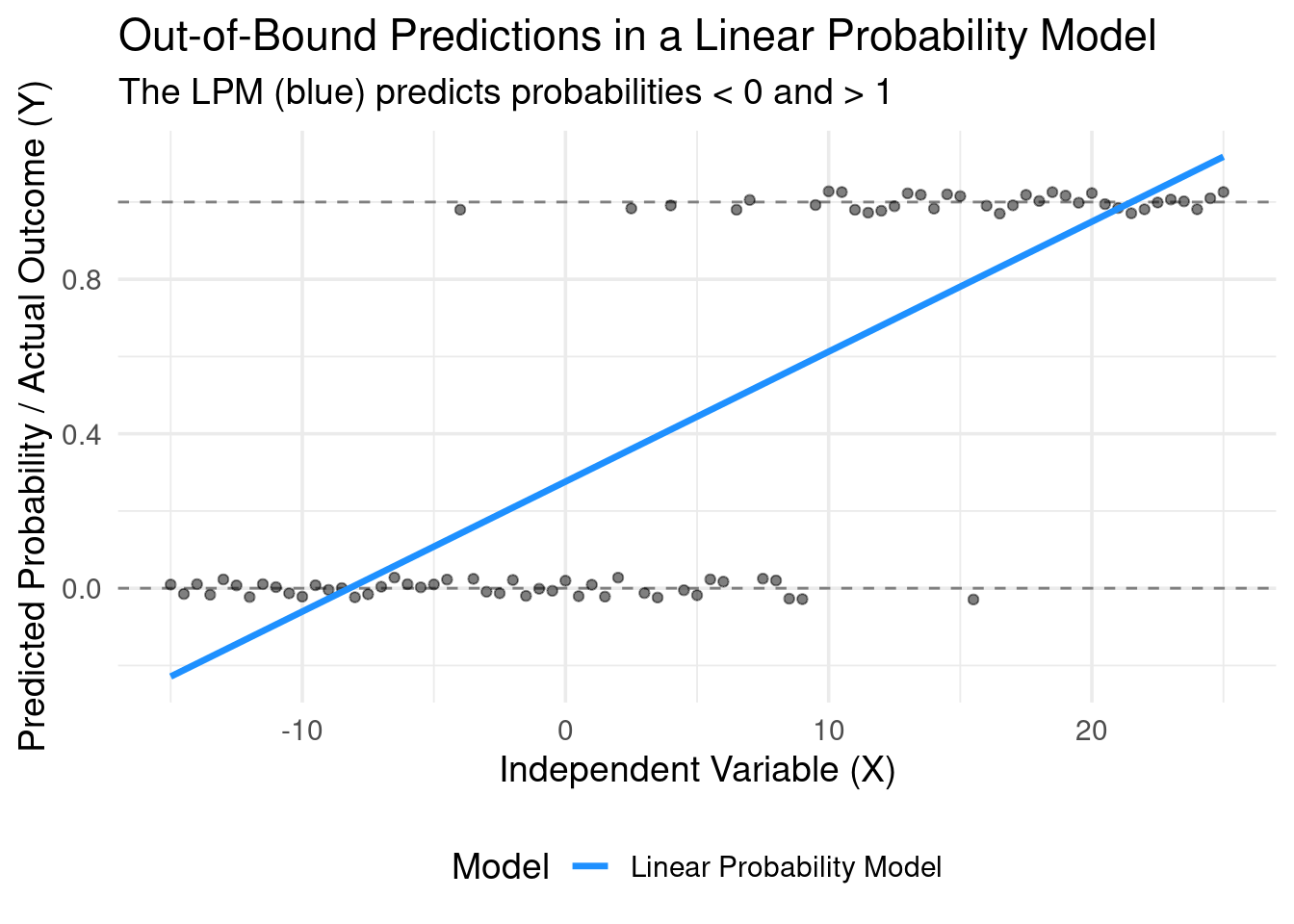
The model is linear, but probability is bounded by \([0, 1]\). The LPM doesn’t know this. \[Pr(y=1|X) = \hat{\beta}_0 + \hat{\beta}_1 X\]
Nothing in the OLS mechanics prevents the predicted value, \(\hat{y}\), from being less than 0 or greater than 1 for certain values of X.
- Interpretation of a predicted probability of 1.2 or -0.1 is nonsensical.
Illustration
Problems with LPM: The Error Term
- The assumptions of the Classical Linear Model are violated.
- The probability that \(y_i=1\) is \(p_i = Pr(y_i=1|X_i)\) is Bernoulli distributed.
- \(E[y_i | X_i] = p_i = \hat{\beta_0} + \hat{\beta_1}x_i\)
- \(Var(y_i | X_i) = p_i(1-p_i)=(\hat{\beta_0} + \hat{\beta_1 x_i}) \cdot (1 - (\hat{\beta_0} + \hat{\beta_1}x_i))\)
- Inherent Heteroskedasticity:
- The variance of the error term depends on the values of the independent variables.
- \(Var(\epsilon_i | X_i) = p_i(1-p_i)\), where \(p_i = Pr(y_i=1|X_i)\)
- Since \(p_i\) depends on X, the variance is not constant. This is heteroskedasticity.
- Consequence: OLS standard errors are biased. We could use robust standard errors to fix this problem.
LPM Summary
Pros: Simple to interpret. It is also easy to incorporate fixed effects in an LPM.
Cons: Nonsensical predictions, violates key OLS assumptions.
We need a model that constrains the predicted probability to be between 0 and 1. We need a non-linear model.
This requires a different way of thinking about the choice process.
Probability Reminder
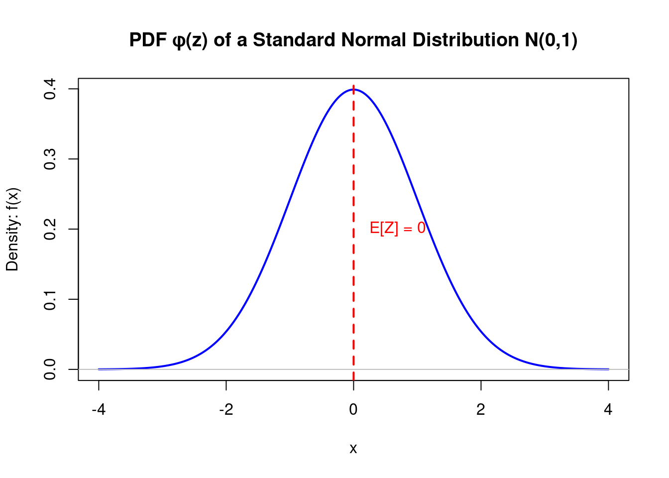
The PDF describes the relative likelihood that a continuous random variable \(Z\) takes on a given value.
For a continuous variable, the probability of it being exactly one value is zero (\(Pr(Z=z) = 0\)). Instead, the PDF gives us a function where the area under the curve over an interval corresponds to the probability of the variable falling within that interval.
- A higher value of \(f_Z(z)\) means that values in that immediate vicinity are more likely to occur.
Formal Properties:
- \(f_Z(z) \ge 0\) for all \(z\). The density is never negative.
- \(\int_{-\infty}^{\infty} f_Z(z) dz = 1\). The total area under the curve is one.
- \(Pr(a \le X \le b) = \int_{a}^{b} f_Z(z) dz\). The probability of \(Z\) being between \(a\) and \(b\) is the area under the PDF from \(a\) to \(b\).
PDF Visualization
CDF
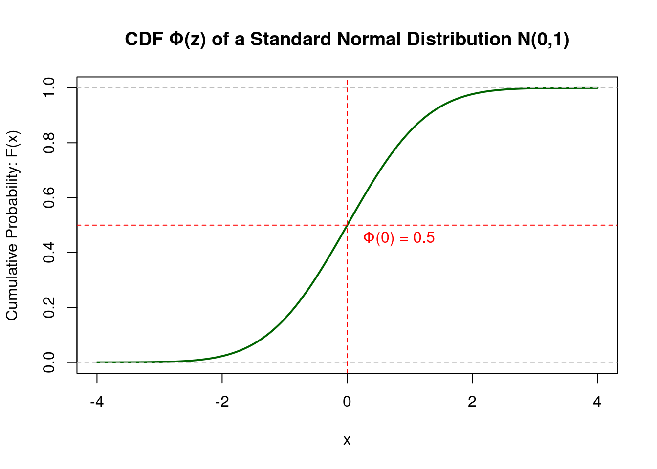
The CDF \(F(z)\) gives the probability that a random variable \(Z\) is less than or equal to a particular value \(z\).
Think of the CDF as a “running total” of the probability. As you move from left to right along the x-axis, it accumulates all the probability up to that point. This is why its value always goes from 0 to 1.
Formal Properties:
- \(F_Z(z) = P(Z \le z)\). This is the definition.
- The CDF is a non-decreasing function of \(x\).
- \(\lim_{z \to -\infty} F_Z(z) = 0\) and \(\lim_{z \to \infty} F_Z(z) = 1\).
- For a continuous variable, \(P(a < Z \le b) = F_Z(b) - F_Z(a)\).
CDF Visualization
Relationship Between PDF and CDF
The PDF and CDF are intrinsically linked. This relationship is foundational for many econometric concepts, including Maximum Likelihood Estimation.
In particular, the PDF is the derivative of the CDF. \[ f_Z(z) = \frac{dF_Z(z)}{dz} \]
- Intuition: The height of the PDF at a point \(z\) represents the slope (or rate of change) of the CDF at that same point. Where the PDF is high (e.g., at the mean), the CDF is steepest, as probability is accumulating most rapidly.
Less importantly here, the CDF is the integral of the PDF.
Why This Matters in Econometrics
The S-shape of the CDF is crucial for modeling probabilities in models like Probit and Logit.
The CDF naturally constrains the output to be between 0 and 1, which is exactly what a probability requires.
The choice of distribution (e.g., Normal for Probit, Logistic for Logit) determines the specific shape of this S-curve.
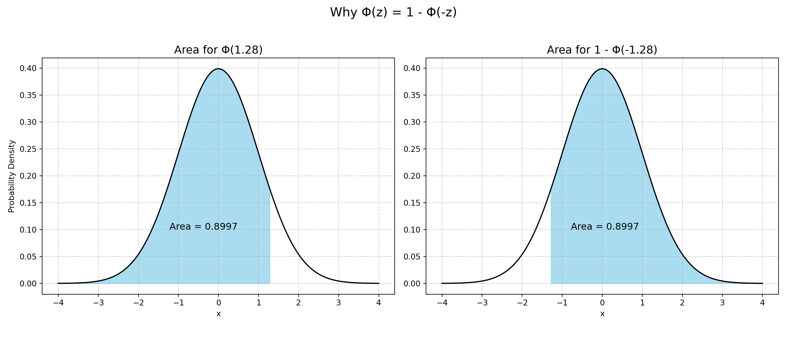
A important property of both the Normal and Logistic CDF: \(1 - F(-z) = F(z)\)
Logit and Probit Models
The Latent Variable Framework
Let’s imagine the binary choice is driven by an unobserved, underlying continuous variable, \(y^*\).
\(y^*\) can be thought of as the “net utility,” “propensity,” or “tendency” to choose 1.
Definition: Latent Variable Framework
\(y_i^* = \beta_0 + \beta_1 x_i + \epsilon_i\)
We don’t observe \(y^*\). We only observe the outcome, y, based on a threshold (usually normalized to 0):
- If \(y_i^* > 0\), then we choose Yes (\(y_i = 1\)), and if \(y_i^* \le 0\), then we choose No (\(y_i = 0\))
The probability that \(y_i=1\) is the probability that \(y_i^*\) is greater than 0.
\[ Pr(y_i=1) = P(y_i^* > 0) = Pr(\beta_0 + \beta_1 x_i + \epsilon_i > 0) = Pr(\epsilon_i > -(\beta_0 + \beta_1 x_i)) \]
\[ Pr(y_i=0) = P(y_i^* \le 0) = Pr(\beta_0 + \beta_1 x_i + \epsilon_i \le 0) = Pr(\epsilon_i \le -(\beta_0 + \beta_1 x_i)) \]
From Latent Variables to Probit & Logit
This links the probability of the observed outcome to the distribution of the unobserved error term, \(\epsilon_i\).
The final step depends on what we assume about the distribution of \(\epsilon_i\).
\[ P(y_i=1) = P(\epsilon_i > -(\beta_0 + \beta_1 x_i)) = 1 - F(-(\beta_0 + \beta_1 x_i)) \]
where F is the Cumulative Distribution Function (CDF) of \(\epsilon_i\).
Probit and Logit
- Two common choices for \(F\) are the normal distribution (Probit model) and the logistic distribution (Logit model)
Definition: Probit and Logit Models
Probit Model: Assumes \(\epsilon_i\) follows a Standard Normal distribution.
- \(P(y_i=1 | X_i) = 1 - \Phi (-(\beta_0 + \beta_1 x_i)) = \Phi(\beta_0 + \beta_1 x_i)\)
- where \(\Phi(\cdot)\) is the Standard Normal CDF.
Logit Model: Assumes \(\epsilon_i\) follows a Standard Logistic distribution.
- \(P(y_i=1 | X_i) = 1 - \Lambda(-(\beta_0 + \beta_1 x_i)) = \Lambda(\beta_0 + \beta_1 x_i) = \frac{e^{\beta_0 + \beta_1 x_i}}{1 + e^{\beta_0 + \beta_1 x_i}}=\frac{1}{1 + e^{-(\beta_0 + \beta_1 x_i)}}\)
- where \(\Lambda(\cdot)\) is the Standard Logistic CDF.
In both cases, \(1-F(-(\beta_0 + \beta_1 x_i)) = F(\beta_0 + \beta_1 x_i)\), since both distributions are symmetric. Both CDFs produce the S-shaped curve we need.
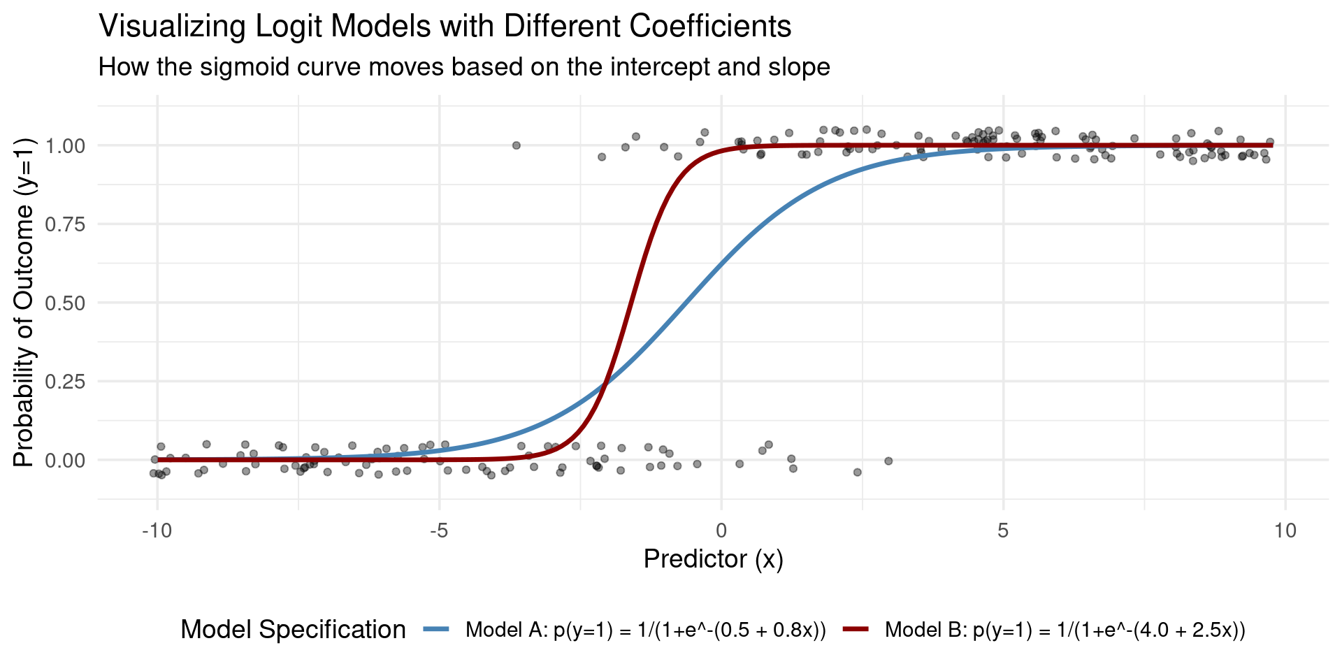
Logistic Function
Definition: Logistic Function
The logistic function, also known as the standard logistic cumulative distribution function (CDF) or sigmoid function, is a function that produces an “S”-shaped curve. It is defined by the formula:
\[ F(x) = \frac{1}{1 + e^{-x}} \]
This function takes any real-valued number and maps it to a value between 0 and 1, making it particularly useful for modeling probabilities.
As it is a CDF, the function always outputs a value between 0 and 1, but never reaches exactly 0 or 1. This makes it ideal for representing probabilities in statistical models like logistic regression.
The standard logistic function is symmetric around the point \((0, 0.5)\). This means that \(F(0) = 0.5\), and the curve is (rotationally) symmetric around this point.
Visualization Logit and Probit Models
Logit and Probit with Panel Data
Panel data allows us to control for unobserved, time-invariant individual characteristics (e.g., innate ability, motivation).
In linear models, this is straightforward. However, the non-linear nature of Logit and Probit models makes this complicated.
Conditional Logit: this model cleverly avoids estimating the fixed effects directly. Instead, it uses a conditional maximum likelihood estimation that focuses only on individuals who change their outcome (switch from 0 to 1 or 1 to 0) at some point in the panel.
- Advantage: Allows for correlation between the unobserved fixed effects and the explanatory variables, just like a standard Fixed Effects model.
- Limitation: Individuals who never change their outcome are dropped from the analysis. It also cannot estimate the effect of time-invariant variables (e.g., gender).
Random Effects Probit: this model treats the unobserved individual effects as random variables that are part of the error term.
- Advantage: It uses all the data (not just the “switchers”) and can estimate the effects of time-invariant variables.
- Limitation: It relies on the strong assumption that the unobserved effects are uncorrelated with the explanatory variables. If this assumption is violated, the estimates will be biased and inconsistent, like RE.
Estimation of Logit and Probit
Estimation: Maximum Likelihood (MLE)
- Remember that in OLS, we take \(\sum (y_i - \hat{y_i} (\beta, x_i))^2\) and set the derivative to zero to express the optimal \(\beta\) coefficients.
- These conditions may not lead to a unique expression for the \(\beta\)-coefficients in Logit/Probit.
- Hence we can’t use OLS. Instead, we use Maximum Likelihood Estimation (MLE).
Definition: Maximum Likelihood Estimation
MLE finds the parameter values (\(\beta\)) that maximize the probability of observing the actual data we collected.
- In other words: “Given our data, what are the most likely parameter values that could have generated it?”
Simple MLE Example: A Biased Coin
Example: A Biased Coin
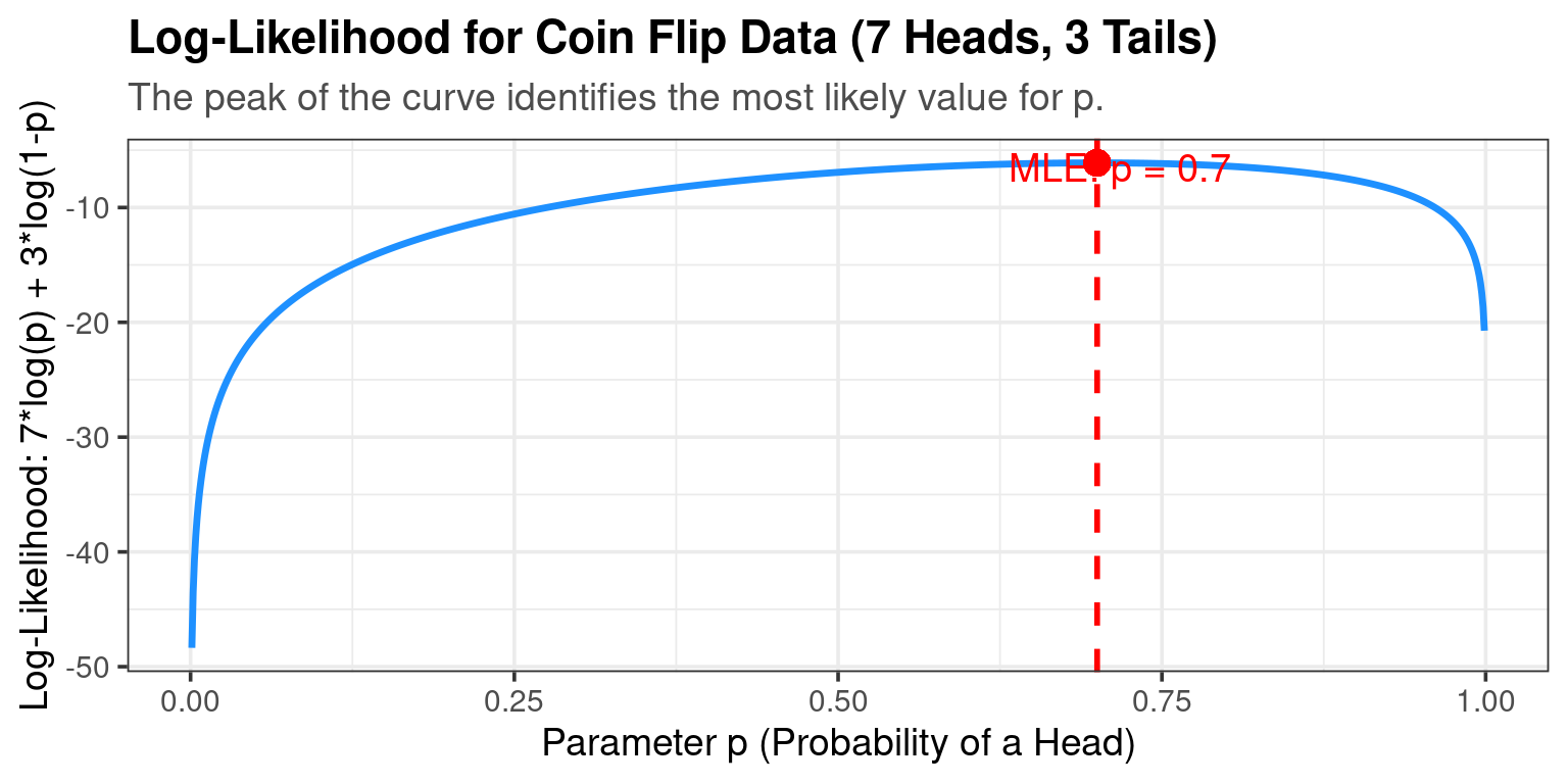
Imagine you flip a coin 10 times and get 7 Heads (H) and 3 Tails (T).
- Data: {H, H, T, H, H, T, H, H, T, H}
- Question: What is your best guess for p, the probability of getting a Head?
The Likelihood Function \(L(p | \text{Data})\): The probability of observing this specific sequence is: \[L(p) = p \cdot p \cdot (1-p) \cdot p \cdot p \cdot (1-p) \cdot p \cdot p \cdot (1-p) \cdot p = p^7 (1-p)^3\]
The goal is to find the value of p that maximizes this function.
- Intuition: Your gut says p = 0.7.
- Optimization: We can take lots of values of \(p\) and calculate the likelihood, and see which value of \(p\) gives us the highest likelihood.
- The result is indeed \(\hat{p}_{MLE} = 0.7\).
This is the value of p that makes the data we saw “most likely.”
MLE Visualization
MLE Visualization: Biased Coin
MLE for Probit/Logit Models
For our regression models, the principle is the same, the calculations are just more complex.
The Likelihood Function is the product of the probabilities of each individual observation: \(L(\beta) = \prod_{i=1}^{N} [P(y_i=1|X_i)]^{y_i} \cdot [1 - P(y_i=1|X_i)]^{1-y_i}\)
- If \(y_i=1\), we use \(P(y_i=1|X_i)\)
- If \(y_i=0\), we use \(1-P(y_i=1|X_i) = P(y_i=0|X_i)\)
We plug in the Probit or Logit formula for \(P(y_i=1|X_i)\) and use a computer to find the \(\beta\) vector that maximizes this function (or more commonly, the log of this function, the Log-Likelihood).
MLE: Probit Example
Example: MLE for Probit
Likelihood Function: \[ \mathcal{L}(\beta) = \prod_{i=1}^n \Phi(\beta_0 + \beta_1 x_i)^{Y_i} [1 - \Phi(\beta_0 + \beta_1 x_i)]^{1-Y_i} \]
Log-Likelihood Function: \[ \log\mathcal{L}(\beta) = \sum_{i=1}^n \left\{ Y_i \log\Phi(\beta_0 + \beta_1 x_i) + (1-Y_i)\log[1-\Phi(\beta_0 + \beta_1 x_i)] \right\} \]
First-Order Conditions (FOC): \[ \frac{\partial \log\mathcal{L}(\beta_0, \dots, \beta_k)}{\partial \beta_j} = \sum_{i=1}^n \left[ \frac{Y_i \phi(\beta_0 + \beta_1 x_{i1} + \dots + \beta_k x_{ik})}{\Phi(\beta_0 + \beta_1 x_{i1} + \dots + \beta_k x_{ik})} - \frac{(1-Y_i)\phi(\beta_0 + \beta_1 x_{i1} + \dots + \beta_k x_{ik})}{1-\Phi(\beta_0 + \beta_1 x_{i1} + \dots + \beta_k x_{ik})} \right] x_{ij} = 0 \]
Interpreting Coefficients
In Probit and Logit models, the estimated coefficients (\(\hat{\beta}\)) are NOT marginal effects.
\[ P(y=1|X) = F(\beta x_i ) \]
A one-unit change in \(x_k\) changes the argument \(\beta x_i\) by \(\beta_k\).
But the change in the probability depends on the slope of the S-curve, which depends on the values of all X variables:
\[ \frac{\partial P(y=1 | x_i)}{\partial x_i} = F'(\beta x_i) \cdot \beta = f(\beta x_i) \cdot \beta \]
This means that the change in the probability does not only depend on \(\beta\), but also on the values of the independent variables \(x_i\) and the function \(F'\).
So, how do we get meaningful interpretations?
Interpretation Method 1: Marginal Effect at the Mean
- We simply calculate the change in predicted probability for a change in an x-variable at a particular value.
Marginal Effect at the Mean
The marginal effect at the mean equals:
\[ \frac{\partial P(y=1|X)}{\partial x_k} = f(\beta \bar{x}) \cdot \beta_k \]
where \(f(\cdot)\) is the PDF, the derivative of the CDF \(F\).
In other words, we simply calculate the MEs with all X variables set to their sample means.
Problem: No single observation in the data might actually have all mean values. “The average person” doesn’t exist.
Interpretation Method 2: Average Marginal Effect
- This is the modern, preferred standard. It gives the best summary of the effect for the population in the sample.
Average Marginal Effect
The Average Marginal Effect (AME) equals:
\[ \frac{\partial P(y=1|X)}{\partial x_k} = \frac{1}{N} \sum_{i=1}^N f(\beta x_i) \cdot \beta_k \]
In other words, we compute the marginal effect using the values of each observations, and then take the average.
Logit and Probit in Software
Example: Bertrand and Mullainathan (2004)
The paper “Are Emily and Greg More Employable Than Lakisha and Jamal?” is a Field Experiment on Labor Market Discrimination”.
They sent thousands of fictitious resumes to real job openings in Boston and Chicago, randomly assigning either a “White-sounding” name or an “African American-sounding” name to otherwise identical resumes.
The study found that resumes with “White-sounding” names received 50% more callbacks for interviews than those with “African American-sounding” names. This racial gap in callbacks was consistent across various occupations, industries, and employer sizes.
The paper provides strong evidence of persistent racial discrimination in the hiring process.
Logit and Probit in Software - Example
- R/Python/Stata have excellent options to run both logistic regression and probit models. Below are some examples on the basis of the Bertrand and Mullainathan (2004) dataset.
Code
df <- haven::read_dta('../../tutorials/datafiles/lakisha_aer.dta')
# LPM
model <- lm(call~ race + sex + C(occupbroad), data=df)
summary(model)
##
## Call:
## lm(formula = call ~ race + sex + C(occupbroad), data = df)
##
## Residuals:
##      Min       1Q   Median       3Q      Max
## -0.13100 -0.09310 -0.07938 -0.05448  0.95426
##
## Coefficients:
##                 Estimate Std. Error t value Pr(>|t|)
## (Intercept)     0.054477   0.007907   6.889 6.32e-12 ***
## racew           0.032564   0.007781   4.185 2.90e-05 ***
## sexm           -0.007658   0.009921  -0.772  0.44024
## C(occupbroad)3  0.043963   0.022373   1.965  0.04947 *
## C(occupbroad)4  0.013719   0.010268   1.336  0.18155
## C(occupbroad)5 -0.008737   0.014527  -0.601  0.54760
## C(occupbroad)6  0.028718   0.010159   2.827  0.00472 **
## ---
## Signif. codes:  0 '***' 0.001 '**' 0.01 '*' 0.05 '.' 0.1 ' ' 1
##
## Residual standard error: 0.2714 on 4863 degrees of freedom
## Multiple R-squared:  0.006335,   Adjusted R-squared:  0.005109
## F-statistic: 5.167 on 6 and 4863 DF,  p-value: 2.63e-05
# Logit
model <- glm(call ~ race + sex + C(occupbroad), data=df, family=binomial(link="logit"))
summary(model)
##
## Call:
## glm(formula = call ~ race + sex + C(occupbroad), family = binomial(link = "logit"),
##     data = df)
##
## Coefficients:
##                Estimate Std. Error z value Pr(>|z|)
## (Intercept)     -2.8232     0.1179 -23.939  < 2e-16 ***
## racew            0.4467     0.1075   4.154 3.27e-05 ***
## sexm            -0.1073     0.1385  -0.775  0.43828
## C(occupbroad)3   0.5475     0.2683   2.040  0.04131 *
## C(occupbroad)4   0.1979     0.1431   1.383  0.16680
## C(occupbroad)5  -0.1375     0.2191  -0.627  0.53040
## C(occupbroad)6   0.3790     0.1354   2.799  0.00513 **
## ---
## Signif. codes:  0 '***' 0.001 '**' 0.01 '*' 0.05 '.' 0.1 ' ' 1
##
## (Dispersion parameter for binomial family taken to be 1)
##
##     Null deviance: 2726.9  on 4869  degrees of freedom
## Residual deviance: 2696.1  on 4863  degrees of freedom
## AIC: 2710.1
##
## Number of Fisher Scoring iterations: 5
# Probit
model <- glm(call ~ race + sex + C(occupbroad), data=df, family=binomial(link="probit"))
summary(model)
##
## Call:
## glm(formula = call ~ race + sex + C(occupbroad), family = binomial(link = "probit"),
##     data = df)
##
## Coefficients:
##                Estimate Std. Error z value Pr(>|z|)
## (Intercept)    -1.58788    0.05668 -28.015  < 2e-16 ***
## racew           0.21908    0.05295   4.138 3.51e-05 ***
## sexm           -0.05431    0.06817  -0.797  0.42565
## C(occupbroad)3  0.26899    0.13923   1.932  0.05336 .
## C(occupbroad)4  0.09471    0.07040   1.345  0.17853
## C(occupbroad)5 -0.06841    0.10497  -0.652  0.51456
## C(occupbroad)6  0.18677    0.06754   2.765  0.00569 **
## ---
## Signif. codes:  0 '***' 0.001 '**' 0.01 '*' 0.05 '.' 0.1 ' ' 1
##
## (Dispersion parameter for binomial family taken to be 1)
##
##     Null deviance: 2726.9  on 4869  degrees of freedom
## Residual deviance: 2696.4  on 4863  degrees of freedom
## AIC: 2710.4
##
## Number of Fisher Scoring iterations: 5
Code
import pandas as pd
import statsmodels.formula.api as smf

df = pd.read_stata('../../tutorials/datafiles/lakisha_aer.dta')
# LPM
model = smf.ols(formula="call ~ race + sex + C(occupbroad)", data=df)
results = model.fit()
print(results.summary())
##                             OLS Regression Results
## ==============================================================================
## Dep. Variable:                   call   R-squared:                       0.006
## Model:                            OLS   Adj. R-squared:                  0.005
## Method:                 Least Squares   F-statistic:                     5.167
## Date:                Wed, 29 Oct 2025   Prob (F-statistic):           2.63e-05
## Time:                        12:56:03   Log-Likelihood:                -555.22
## No. Observations:                4870   AIC:                             1124.
## Df Residuals:                    4863   BIC:                             1170.
## Df Model:                           6
## Covariance Type:            nonrobust
## ======================================================================================
##                          coef    std err          t      P>|t|      [0.025      0.975]
## --------------------------------------------------------------------------------------
## Intercept              0.0545      0.008      6.889      0.000       0.039       0.070
## race[T.w]              0.0326      0.008      4.185      0.000       0.017       0.048
## sex[T.m]              -0.0077      0.010     -0.772      0.440      -0.027       0.012
## C(occupbroad)[T.3]     0.0440      0.022      1.965      0.049       0.000       0.088
## C(occupbroad)[T.4]     0.0137      0.010      1.336      0.182      -0.006       0.034
## C(occupbroad)[T.5]    -0.0087      0.015     -0.601      0.548      -0.037       0.020
## C(occupbroad)[T.6]     0.0287      0.010      2.827      0.005       0.009       0.049
## ==============================================================================
## Omnibus:                     2957.734   Durbin-Watson:                   1.449
## Prob(Omnibus):                  0.000   Jarque-Bera (JB):            18742.316
## Skew:                           3.055   Prob(JB):                         0.00
## Kurtosis:                      10.418   Cond. No.                         7.27
## ==============================================================================
##
## Notes:
## [1] Standard Errors assume that the covariance matrix of the errors is correctly specified.

# Logit
model = smf.logit(formula="call ~ race + sex + C(occupbroad)", data=df)
results = model.fit()
## Optimization terminated successfully.
##          Current function value: 0.276811
##          Iterations 7
print(results.summary())
##                            Logit Regression Results
## ==============================================================================
## Dep. Variable:                   call   No. Observations:                 4870
## Model:                          Logit   Df Residuals:                     4863
## Method:                           MLE   Df Model:                            6
## Date:                Wed, 29 Oct 2025   Pseudo R-squ.:                 0.01129
## Time:                        12:56:03   Log-Likelihood:                -1348.1
## converged:                       True   LL-Null:                       -1363.5
## Covariance Type:            nonrobust   LLR p-value:                 2.792e-05
## ======================================================================================
##                          coef    std err          z      P>|z|      [0.025      0.975]
## --------------------------------------------------------------------------------------
## Intercept             -2.8232      0.118    -23.939      0.000      -3.054      -2.592
## race[T.w]              0.4467      0.108      4.154      0.000       0.236       0.657
## sex[T.m]              -0.1073      0.138     -0.775      0.438      -0.379       0.164
## C(occupbroad)[T.3]     0.5475      0.268      2.040      0.041       0.022       1.073
## C(occupbroad)[T.4]     0.1979      0.143      1.383      0.167      -0.083       0.478
## C(occupbroad)[T.5]    -0.1375      0.219     -0.627      0.530      -0.567       0.292
## C(occupbroad)[T.6]     0.3790      0.135      2.799      0.005       0.114       0.644
## ======================================================================================

# Probit
model = smf.probit(formula="call ~ race + sex + C(occupbroad)", data=df)
results = model.fit()
## Optimization terminated successfully.
##          Current function value: 0.276840
##          Iterations 6
print(results.summary())
##                           Probit Regression Results
## ==============================================================================
## Dep. Variable:                   call   No. Observations:                 4870
## Model:                         Probit   Df Residuals:                     4863
## Method:                           MLE   Df Model:                            6
## Date:                Wed, 29 Oct 2025   Pseudo R-squ.:                 0.01119
## Time:                        12:56:03   Log-Likelihood:                -1348.2
## converged:                       True   LL-Null:                       -1363.5
## Covariance Type:            nonrobust   LLR p-value:                 3.154e-05
## ======================================================================================
##                          coef    std err          z      P>|z|      [0.025      0.975]
## --------------------------------------------------------------------------------------
## Intercept             -1.5879      0.056    -28.175      0.000      -1.698      -1.477
## race[T.w]              0.2191      0.053      4.138      0.000       0.115       0.323
## sex[T.m]              -0.0543      0.068     -0.797      0.425      -0.188       0.079
## C(occupbroad)[T.3]     0.2690      0.139      1.931      0.054      -0.004       0.542
## C(occupbroad)[T.4]     0.0947      0.070      1.344      0.179      -0.043       0.233
## C(occupbroad)[T.5]    -0.0684      0.105     -0.652      0.514      -0.274       0.137
## C(occupbroad)[T.6]     0.1868      0.067      2.769      0.006       0.055       0.319
## ======================================================================================Marginal Effects in Software
- R/Python/Stata have libraries that allow you to calculate the marginal effects in these two ways easily.
Code
library(marginaleffects)
# Model as before
# Logit
model <- glm(call ~ race + sex + C(occupbroad), data=df, family=binomial(link="logit"))

# Using the marginaleffects package
avg_slopes(model, variables = c('race', 'sex'))
##
##  Term Contrast Estimate Std. Error      z Pr(>|z|)    S   2.5 % 97.5 %
##  race    w - b   0.0326    0.00778  4.187   <0.001 15.1  0.0173 0.0478
##  sex     m - f  -0.0077    0.00970 -0.794    0.427  1.2 -0.0267 0.0113
##
## Type: response
Code
import statsmodels.formula.api as smf
# Logit
model = smf.logit(formula="call ~ race + sex + C(occupbroad)", data=df)
results = model.fit()
## Optimization terminated successfully.
##          Current function value: 0.276811
##          Iterations 7

# Using the `get.margeff` method:
results.get_margeff(at='overall').summary_frame()
##                        dy/dx  Std. Err.  ...  Conf. Int. Low  Cont. Int. Hi.
## race[T.w]           0.032848   0.007982  ...        0.017204        0.048492
## sex[T.m]           -0.007892   0.010186  ...       -0.027856        0.012071
## C(occupbroad)[T.3]  0.040260   0.019773  ...        0.001506        0.079014
## C(occupbroad)[T.4]  0.014551   0.010536  ...       -0.006099        0.035201
## C(occupbroad)[T.5] -0.010109   0.016116  ...       -0.041697        0.021479
## C(occupbroad)[T.6]  0.027870   0.009998  ...        0.008274        0.047465
##
## [6 rows x 6 columns]
results.get_margeff(at='mean').summary_frame()
##                        dy/dx  Std. Err.  ...  Conf. Int. Low  Cont. Int. Hi.
## race[T.w]           0.032075   0.007592  ...        0.017196        0.046954
## sex[T.m]           -0.007707   0.009937  ...       -0.027182        0.011769
## C(occupbroad)[T.3]  0.039313   0.019207  ...        0.001668        0.076957
## C(occupbroad)[T.4]  0.014208   0.010256  ...       -0.005893        0.034310
## C(occupbroad)[T.5] -0.009871   0.015725  ...       -0.040692        0.020950
## C(occupbroad)[T.6]  0.027213   0.009656  ...        0.008288        0.046139
##
## [6 rows x 6 columns]
Code
* Logit
logit call race sex i.occupbroad

* Calculate the Average Marginal Effect for all variables
margins, dydx(*)

* Calculate the Marginal Effect at the Mean for all variables
margins, dydx(*) atmeans
* The interpretation is similar to the AME, but it applies specifically to an observation with average characteristics rather than being an average of individual effects.
Goodness-of-Fit and Testing
How well does our model fit the data?
Percent Correctly Predicted:
- If \(\hat{p}_i > 0.5\), predict \(y=1\). If \(\hat{p}_i \le 0.5\), predict \(y=0\).
- Compare predictions to actual outcomes. What percentage did we get right?
- Intuitive, but sensitive to the 0.5 cutoff.
Pseudo R-Squared:
- Several versions exist, like McFadden’s R-squared.
- \(R^2_{McF} = 1 - \frac{\ln L_{full}}{\ln L_{null}}\) (where \(L_{null}\) is from a model with only an intercept).
- Ranges from 0 to 1, but values are much lower than OLS R-squared. A value of 0.2-0.4 can indicate a very good fit. Do not compare to OLS R-squared!
Likelihood Ratio (LR) Test:
- Tests the joint significance of a set of variables (like the F-test in OLS).
- Compares the log-likelihood of the restricted model to the unrestricted (full) model.
- \(LR = 2(\ln L_{full} - \ln L_{restricted})\) which follows a \(\chi^2\) distribution.
Predictive Accuracy: The Confusion Matrix
- This is the most intuitive method for assessing a model’s performance. It’s based on how well the model classifies individual cases.
- The model calculates a predicted probability, \(\hat{p}_i\), for each observation.
- We choose a classification threshold (commonly 0.5).
- We classify the prediction: if \(\hat{p}_i > 0.5\), predict 1 (e.g., “Yes”); if \(\hat{p}_i \le 0.5\), predict 0 (e.g., “No”).
- We compare these predictions to the actual outcomes in a “confusion matrix.”
| Predicted: No (0) | Predicted: Yes (1) | |
|---|---|---|
| Actual: No (0) | True Negatives (TN) | False Positives (FP) |
| Actual: Yes (1) | False Negatives (FN) | True Positives (TP) |
- Percent Correctly Predicted (Accuracy) = \(\tfrac{TN + TP}{\text{Total Observations}}\)
- Pro: Very easy to understand and communicate.
- Con: It is highly sensitive to the 0.5 cutoff. If the model is for a rare event (e.g., disease diagnosis), a different threshold might be more appropriate. It also treats all misclassifications as equal.
Calculating Percent Correctly Predicted
- Let’s see how to implement this in code. We will fit a model and then evaluate its accuracy using a confusion matrix.
Code
# Load necessary library for more detailed metrics
# install.packages("caret")
library(caret)

# Create some sample data
set.seed(123) # for reproducibility
sample_data <- data.frame(
  predictor = rnorm(100),
  outcome = rbinom(100, 1, 0.5)
)

# Fit the logistic regression model
logit_model <- glm(outcome ~ predictor, data = sample_data, family = "binomial")

# Get predicted probabilities
predicted_probs <- predict(logit_model, type = "response")

# Convert probabilities to classes (0 or 1) using a 0.5 threshold
predicted_class <- factor(ifelse(predicted_probs > 0.5, 1, 0))
actual_class <- factor(sample_data$outcome)

# Generate the confusion matrix
# 'positive="1"' tells the function which outcome is the "success" class
conf_matrix <- confusionMatrix(data = predicted_class, reference = actual_class, positive="1")

print(conf_matrix)
## Confusion Matrix and Statistics
##
##           Reference
## Prediction  0  1
##          0 37 34
##          1 15 14
##
##                Accuracy : 0.51
##                  95% CI : (0.408, 0.6114)
##     No Information Rate : 0.52
##     P-Value [Acc > NIR] : 0.61838
##
##                   Kappa : 0.0033
##
##  Mcnemar's Test P-Value : 0.01013
##
##             Sensitivity : 0.2917
##             Specificity : 0.7115
##          Pos Pred Value : 0.4828
##          Neg Pred Value : 0.5211
##              Prevalence : 0.4800
##          Detection Rate : 0.1400
##    Detection Prevalence : 0.2900
##       Balanced Accuracy : 0.5016
##
##        'Positive' Class : 1
##
Code
import pandas as pd
import numpy as np
from sklearn.linear_model import LogisticRegression
from sklearn.metrics import confusion_matrix, classification_report

# 1. Create some sample data
np.random.seed(123) # for reproducibility
sample_data = pd.DataFrame({
    'predictor': np.random.randn(100),
    'outcome': np.random.binomial(1, 0.5, 100)
})

# Define predictor (X) and outcome (y) variables
# We need to reshape the predictor to be a 2D array for scikit-learn
X = sample_data[['predictor']]
y = sample_data['outcome']

# 2. Fit the logistic regression model
logit_model = LogisticRegression()
model_fit = logit_model.fit(X, y)

# 3. Get predicted classes
# .predict() automatically uses a 0.5 probability threshold
predicted_class = model_fit.predict(X)

# 4. Generate the confusion matrix and classification report
# The labels parameter ensures the matrix is in the order [0, 1]
# for TN, FP, FN, TP
conf_matrix = confusion_matrix(y_true=y, y_pred=predicted_class)
print(conf_matrix)
## [[13 30]
##  [ 8 49]]
# The classification_report provides precision, recall, f1-score, etc.
class_report = classification_report(y_true=y, y_pred=predicted_class)
print(class_report)
##               precision    recall  f1-score   support
##
##            0       0.62      0.30      0.41        43
##            1       0.62      0.86      0.72        57
##
##     accuracy                           0.62       100
##    macro avg       0.62      0.58      0.56       100
## weighted avg       0.62      0.62      0.59       100
Code
* Clear any existing data and set seed for reproducibility
clear all
set seed 123

* 1. Create some sample data
* Set the number of observations to 100
set obs 100

* Generate the predictor variable from a standard normal distribution
gen predictor = rnormal()

* Generate the binary outcome variable from a binomial distribution
* This creates a variable that is 0 or 1, with a 60% probability of being 1
gen outcome = rbinomial(1, 0.6)


* 2. Fit the logistic regression model
* The command 'logit' runs the model with 'outcome' as the dependent variable
logit outcome predictor


* 3. Generate the confusion matrix and classification report
* The 'estat classification' command is run immediately after the regression.
* It automatically uses a 0.5 probability threshold to classify outcomes.
estat classification
The output from the confusion matrix gives a detailed breakdown, including the confusion matrix itself, and key metrics like:
- Accuracy: The overall “Percent Correctly Predicted.”
- Sensitivity: The proportion of actual positives that were correctly identified.
- Specificity: The proportion of actual negatives that were correctly identified.
Explanatory Power: Pseudo R-Squared
In linear regression, \(R^2\) tells us the proportion of variance explained by the model. We can’t use the same metric for logistic regression, but we have alternatives called Pseudo R-Squareds.
McFadden’s \(R^2\) is a common choice. It is based on the log-likelihood of two models:
- The Full Model (\(L_{full}\)): The model with all of our chosen predictors.
- The Null Model (\(L_{null}\)): A basic model with only an intercept. This model essentially predicts the same probability (the overall sample proportion) for every observation.
\[ R^2_{McF} = 1 - \frac{\ln L_{full}}{\ln L_{null}} \]
Interpretation:
- Ranges from 0 to 1: A value of 0 means your predictors are useless. A value of 1 would mean a perfect fit.
- Values are much lower than OLS R-squared: Do not make a direct comparison! A McFadden’s \(R^2\) between 0.2 and 0.4 can indicate a very good model fit.
- It represents the improvement in the log-likelihood of the full model compared to the null model.
The Likelihood Ratio (LR) Test
The LR test is the equivalent of the F-test in OLS.
- It tests the joint significance of a set of variables by comparing the goodness-of-fit of two nested models.
- One model (the restricted model) is a special case of the other (the full model). For example, a model with predictors \(X_1\) is nested within a model with predictors \((X_1, X_2)\).
- The test determines if the additional variables in the full model provide a statistically significant improvement in fit compared to the simpler, restricted model. \(LR = 2(\ln L_{full} - \ln L_{restricted})\)
This statistic follows a Chi-Squared (\(\chi^2\)) distribution, with degrees of freedom equal to the number of variables excluded from the restricted model.
- \(H_0\) (Null Hypothesis): The restricted model is the true model. The coefficients of the extra variables in the full model are all equal to zero.
- \(H_A\) (Alternative Hypothesis): The full model is the true model. At least one of the extra variables has a non-zero coefficient.
- A small p-value (< 0.05) rejects \(H_0\).
- It suggests that the full model is a significant improvement, and the additional variables are jointly significant.
Performing a Likelihood Ratio Test
- A common use of the LR test is to check if the full model is a significant improvement over the null (intercept-only) model.
Code
# Load the library for the LR test
# install.packages("lmtest")
library(lmtest)

# Create the restricted (null) model
null_model <- glm(outcome ~ 1, data = sample_data, family = "binomial")

# Compare the two models using the Likelihood Ratio Test
lr_test_result <- lrtest(null_model, logit_model)

print(lr_test_result)
## Likelihood ratio test
##
## Model 1: outcome ~ 1
## Model 2: outcome ~ predictor
##   #Df  LogLik Df  Chisq Pr(>Chisq)
## 1   1 -69.235
## 2   2 -68.921  1 0.6282      0.428
Code
import pandas as pd
import numpy as np
import statsmodels.api as sm
from scipy.stats import chi2

# --- Setup: Re-creating the data from the previous step ---
# This ensures the script is self-contained.
np.random.seed(123) # for reproducibility
sample_data = pd.DataFrame({
    'predictor': np.random.randn(100),
    'outcome': np.random.binomial(1, 0.5, 100)
})

# Define predictor (X) and outcome (y) variables
y = sample_data['outcome']
X = sample_data[['predictor']]

# In statsmodels, you need to manually add a constant (intercept) to the model
X_with_const = sm.add_constant(X)

# --- Step 1: Fit the full (unrestricted) logistic regression model ---
# This is the same as 'logit_model' from the R code
full_model = sm.Logit(y, X_with_const).fit(disp=0) # disp=0 suppresses convergence messages

# --- Step 2: Fit the restricted (null) model ---
# This model only includes an intercept (outcome ~ 1)
# The predictor is just a column of ones (the constant)
X_null = sm.add_constant(pd.DataFrame({'dummy': np.ones(len(y))})) # Creates just an intercept
null_model = sm.Logit(y, X_null).fit(disp=0)

# --- Step 3: Compare the two models using the Likelihood Ratio Test ---
from scipy.stats.distributions import chi2
def likelihood_ratio(llmin, llmax):
    return(2*(llmax-llmin))

LR = likelihood_ratio(null_model.llf, full_model.llf)
p = chi2.sf(LR, 1) # L2 has 1 DoF more than L1

print('p: %.30f' % p)
## p: 0.109058502086434874756015744879
Code
* Clear any existing data and set seed for reproducibility
clear all
set seed 123

* --- Setup: Re-creating the data from the previous step ---
* This ensures the script is self-contained.
set obs 100
gen predictor = rnormal()
gen outcome = rbinomial(1, 0.6)


* --- Step 1: Fit the full (unrestricted) logistic regression model ---
* This is the model including our variable of interest.
logit outcome predictor

* --- Step 2: Store the estimation results of the full model ---
* The 'estimates store' command saves all the results (like the log-likelihood)
* of the most recent model under a name you choose.
estimates store full_model


* --- Step 3: Fit the restricted (null) model ---
* To fit an intercept-only model, you just specify the dependent variable.
logit outcome


* --- Step 4: Compare the two models using the Likelihood Ratio Test ---
* The 'lrtest' command compares the currently active model (the null model)
* with a previously stored model (full_model).
lrtest full_model
LogLik: The log-likelihood values for the null (Model 1) and full (Model 2) models.
Chisq: This is the LR test statistic (0.5065).
Pr(>Chisq): This is the p-value (0.4766).
Since the p-value is large, we do not reject the null hypothesis. This indicates that our predictor does not provide a statistically significant improvement over a model that simply predicts the mean.
Choosing Between Probit and Logit
- In practice, the choice rarely matters much.
- The Normal and Logistic distributions are very similar, except the Logistic has slightly “fatter tails” (it’s less sensitive to outliers).
- Predicted probabilities from both models are usually very close.
- Rule of Thumb:
- Logit coefficients are larger than Probit coefficients by a factor of ~1.6 - 1.8.
- Logit Marginal Effects \(\approx\) Probit Marginal Effects.
Prediction
Prediction on Unseen Data
Once a model is estimated, its primary purpose is often to make predictions on new data where the outcome is unknown.
The LPM is simply an OLS linear regression model where the dependent variable (Y) is binary (0 or 1).
\[ Y = \beta_0 + \beta_1X_1 + \dots + \beta_kX_k + \epsilon \]
The predicted value, \(\hat{Y}\), is interpreted as the predicted probability of the event occurring (\(P(Y=1)\)).
- To predict on new data, you simply plug the new values of the predictor variables (\(X_i\)) into the estimated regression equation.
- Because the LPM is a simple linear model, its predictions are not bounded between 0 and 1. It is possible—and common—to get predicted “probabilities” that are negative or greater than 1, which are nonsensical.
Predicting in Software
Code
# Create some sample data for training
set.seed(42)
age = sample(20:70, 100, replace = TRUE)

train_data <- data.frame(
  age = age,
  purchased = rbinom(100, 1, prob = age/70)
)

# Fit the Linear Probability Model on the training data
lpm_model <- lm(purchased ~ age, data = train_data)
summary(lpm_model)
##
## Call:
## lm(formula = purchased ~ age, data = train_data)
##
## Residuals:
##     Min      1Q  Median      3Q     Max
## -0.8862 -0.4362  0.1365  0.3176  0.5666
##
## Coefficients:
##             Estimate Std. Error t value Pr(>|t|)
## (Intercept) 0.195708   0.137365   1.425 0.157412
## age         0.011319   0.002823   4.009 0.000119 ***
## ---
## Signif. codes:  0 '***' 0.001 '**' 0.01 '*' 0.05 '.' 0.1 ' ' 1
##
## Residual standard error: 0.4204 on 98 degrees of freedom
## Multiple R-squared:  0.1409, Adjusted R-squared:  0.1321
## F-statistic: 16.07 on 1 and 98 DF,  p-value: 0.000119

# Create new, "unseen" data for which we want to make predictions
unseen_data <- data.frame(
  age = c(18, 25, 45, 68, 85) # Note the ages outside the original range
)

# Use the predict() function to get predicted probabilities
unseen_data$predicted_prob_lpm <- predict(lpm_model, newdata = unseen_data)

print(unseen_data)
##   age predicted_prob_lpm
## 1  18          0.3994487
## 2  25          0.4786810
## 3  45          0.7050590
## 4  68          0.9653938
## 5  85          1.1578152
Code
import pandas as pd
import numpy as np
import statsmodels.api as sm
import statsmodels.formula.api as smf

# 1. Create some sample data for training
np.random.seed(42) # for reproducibility

# R's rbinom recycles the probability vector. We replicate that behavior here.
age = np.random.randint(20, 71, 100) # np.randint is exclusive of the high end
prob_vector = [np.random.binomial(1, i/70, 1)[0] for i in age]# creates a vector of 50 probabilities

train_data = pd.DataFrame({
  'age': age,
  'purchased': prob_vector
})

# 2. Fit the Linear Probability Model (LPM) on the training data
# The formula syntax 'purchased ~ age' is identical to R's
lpm_model = smf.ols('purchased ~ age', data=train_data).fit()

# Print a summary of the model, similar to R's summary()
print("--- Linear Probability Model Summary ---")
## --- Linear Probability Model Summary ---
print(lpm_model.summary())
##                             OLS Regression Results
## ==============================================================================
## Dep. Variable:              purchased   R-squared:                       0.269
## Model:                            OLS   Adj. R-squared:                  0.261
## Method:                 Least Squares   F-statistic:                     35.98
## Date:                Wed, 29 Oct 2025   Prob (F-statistic):           3.34e-08
## Time:                        12:56:06   Log-Likelihood:                -50.800
## No. Observations:                 100   AIC:                             105.6
## Df Residuals:                      98   BIC:                             110.8
## Df Model:                           1
## Covariance Type:            nonrobust
## ==============================================================================
##                  coef    std err          t      P>|t|      [0.025      0.975]
## ------------------------------------------------------------------------------
## Intercept     -0.0717      0.130     -0.551      0.583      -0.330       0.187
## age            0.0166      0.003      5.999      0.000       0.011       0.022
## ==============================================================================
## Omnibus:                       14.238   Durbin-Watson:                   2.004
## Prob(Omnibus):                  0.001   Jarque-Bera (JB):                5.001
## Skew:                          -0.238   Prob(JB):                       0.0821
## Kurtosis:                       2.013   Cond. No.                         151.
## ==============================================================================
##
## Notes:
## [1] Standard Errors assume that the covariance matrix of the errors is correctly specified.
print("\n" + "="*80 + "\n") # Separator for clarity
##
## ================================================================================

# 3. Create new, "unseen" data for which we want to make predictions
unseen_data = pd.DataFrame({
  'age': [18, 25, 45, 68, 85]
})

# 4. Use the .predict() method to get predicted probabilities
# This is the direct equivalent of predict(model, newdata=...)
unseen_data['predicted_prob_lpm'] = lpm_model.predict(unseen_data)

# 5. Print the final predictions
print("--- Predictions on Unseen Data ---")
## --- Predictions on Unseen Data ---
print(unseen_data)
##    age  predicted_prob_lpm
## 0   18            0.226496
## 1   25            0.342466
## 2   45            0.673810
## 3   68            1.054856
## 4   85            1.336498
Code
// 1. Create some sample data for training
clear // Clears any existing data from memory
set obs 100 // Sets the number of observations to 100

// Set the seed for reproducibility, equivalent to np.random.seed(42)
set seed 42

// Generate a variable 'age' with random integers between 20 and 70.
generate age = runiformint(20, 70)

// Generate the 'purchased' variable based on a binomial distribution.

generate purchased = rbinomial(1, age/70)


// 2. Fit the Linear Probability Model (LPM) on the training data
// The 'regress' command fits an OLS model. The dependent variable
// comes first, followed by the independent variable(s).
regress purchased age

// We can store the estimation results for later use if needed.
estimates store lpm_model


// 3. Create new, "unseen" data for which we want to make predictions
clear // Clear the training data to create the new dataset

// Input the new "unseen" data for the 'age' variable.
input age
    18
    25
    45
    68
    85
end // Finalizes the data input


// 4. Use the .predict() command to get predicted probabilities
predict predicted_prob_lpm

// 5. Print the final predictions
list age predicted_prob_lpm- This output clearly illustrates the main weakness of the LPM: for plausible but extreme values of the predictor variables (like an age of 85), the model can predict probabilities outside of the logical range.
Prediction with Logit
The Logit model solves the prediction problem of the LPM by using a logistic function to ensure that predicted probabilities are always between 0 and 1.
The model predicts the natural logarithm of the odds of the event occurring:
\[ \ln\left(\frac{P(Y=1)}{1-P(Y=1)}\right) = \beta_0 + \beta_1X_1 + \dots + \beta_kX_k \]
To get the predicted probability, we solve for \(P(Y=1)\).
- Predict the Log-Odds: The model first calculates the predicted log-odds (the “link”) for the new data.
- Convert to Probability: The log-odds are then transformed into a probability using the logistic function: \(P(Y=1) = \frac{e^{\text{log-odds}}}{1 + e^{\text{log-odds}}}\)
In software, this happens automatically.
Logit Prediction in Software
Code
# Use the same training data as before
# train_data <- data.frame(...)

# Fit the logistic regression model on the training data
logit_model <- glm(purchased ~ age, data = train_data, family = "binomial")

# Use the same "unseen" data
# unseen_data <- data.frame(age = c(18, 25, 45, 68, 85))

# Predict the log-odds (the default)
unseen_data$predicted_log_odds <- predict(logit_model, newdata = unseen_data, type = "link")

# Predict the probability directly
# The 'type = "response"' argument handles the conversion for us
unseen_data$predicted_prob_logit <- predict(logit_model, newdata = unseen_data, type = "response")

# We can also generate a class prediction using a 0.5 threshold
unseen_data$predicted_class <- ifelse(unseen_data$predicted_prob_logit > 0.5, "Purchase", "No Purchase")

print(unseen_data)
##   age predicted_prob_lpm predicted_log_odds predicted_prob_logit
## 1  18          0.3994487         -0.5995532            0.3544459
## 2  25          0.4786810         -0.1776214            0.4557110
## 3  45          0.7050590          1.0278981            0.7365082
## 4  68          0.9653938          2.4142454            0.9179072
## 5  85          1.1578152          3.4389369            0.9688995
##   predicted_class
## 1     No Purchase
## 2     No Purchase
## 3        Purchase
## 4        Purchase
## 5        Purchase
Code
import pandas as pd
import numpy as np
import statsmodels.api as sm
import statsmodels.formula.api as smf

# 1. Estimate logit model
model = smf.logit("purchased ~ age", data=train_data).fit()
## Optimization terminated successfully.
##          Current function value: 0.482057
##          Iterations 6

# 2. Create the unseen data
# --- 2. Use the same "unseen" data ---
unseen_data = pd.DataFrame({
  'age': [18, 25, 45, 68, 85]
})

# 3. Put the data inside an Array for Prediction
X_unseen = unseen_data[['age']]

# 4. Use the predict method to find the predicted probabilities
predicted_probabilities = model.predict(X_unseen)
unseen_data['predicted_prob_logit'] = predicted_probabilities

# 5. Make the prediction on the basis of the 0.5 cutoff
unseen_data['predicted_class'] = np.where(predicted_probabilities > 0.5, "Purchase", "No Purchase")
print(unseen_data)
##    age  predicted_prob_logit predicted_class
## 0   18              0.169488     No Purchase
## 1   25              0.288152     No Purchase
## 2   45              0.741244        Purchase
## 3   68              0.964524        Purchase
## 4   85              0.993078        Purchase
Code
* --- 1. Fit the logistic regression model on the training data ---
logit purchased age

* --- 2. Create new, "unseen" data for which we want to make predictions ---

* Clear the training data (it's safe because of the 'preserve' command)
clear

* Input the new ages for the unseen data directly
input age
18
25
45
68
85
end

* --- 3. Use the 'predict' command to find the predicted probabilities ---

* 'predict' uses the coefficients from the last model that was fit (the logit model).
* The 'pr' option specifies that we want the probability of a positive outcome.
predict predicted_prob_logit, pr

* --- 4. Make the prediction on the basis of the 0.5 cutoff ---

* The cond() function is a direct equivalent of Python's np.where() or R's ifelse().
* It creates a new string variable based on the condition.
gen predicted_class = cond(predicted_prob_logit > 0.5, "Purchase", "No Purchase")

* --- 5. Print the final results ---
* 'list' displays the data currently in memory, now containing the predictions.
* We drop the probability column to exactly match the final Python output.
drop predicted_prob_logit
display "" // Add a blank line for readability
display "--- Logistic Regression Predictions on Unseen Data ---"
list, noobs // The 'noobs' option hides observation numbers for a cleaner look

* --- (Optional but good practice) Restore the original training data ---
restore- Notice how even for the extreme age of 85, the predicted probability from the logit model is 0.99—very high, but logically bounded within the range.
- This makes the logit model a much more robust choice for prediction in binary outcome scenarios.
Limited Dependent Variable Models
Dealing with Truncated Data
- We use Probit and Logit when the outcome we care about is a simple “Yes/No” or “0/1” decision.
- Our variable can also be bounded in other ways.
- Consider annual household spending on a new car. Many households will spend $0.
- For those who do buy, spending will be a positive, continuous amount ($20,000, $35,000, etc.). This is called a censored dependent variable: we have a pile of observations at a specific value (zero) and a continuous distribution for the rest.
- The Tobit model is designed for situations where the dependent variable is censored.
- In this case, OLS would give biased results, and Probit/Logit can’t handle the continuous positive values.
Illustration: Censored Data
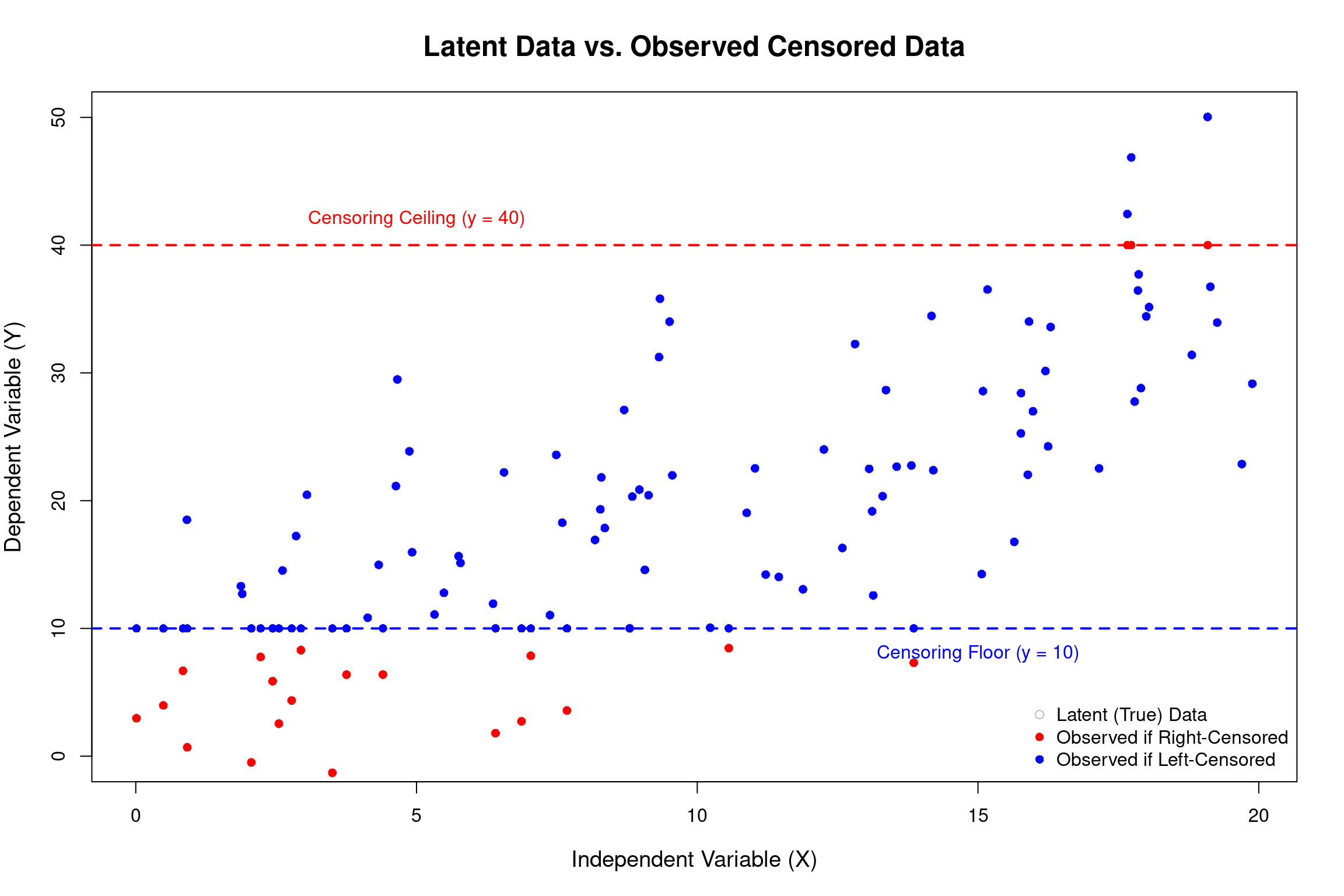
The Tobit Model (Censored Dependent Variable)
- The Tobit model is used when the dependent variable is continuous over a certain range but has a significant number of observations “piled up” at a lower (or upper) limit.
Example: Censored Data
Annual hours worked. Many individuals choose not to work, so their hours are 0. For those who do work, the hours are positive and continuous.
Household expenditure on a durable good (e.g., a car).
A firm’s R&D spending.
Latent Variable Framework
The Tobit model assumes a single underlying decision process. Just as in the logit/probit case, we model a latent (unobserved) variable, \(y^*\), which represents the true desired level or propensity.
\[ y_i^* = β_0 + β_1X_{1i} + β_2X_{2i} + ... + u_i, \text{ where } u_i \sim N(0, \sigma^2) \]
\(y_i^*\) can be thought of as the “desired hours of work” or “propensity to spend.” It can be negative.
Observation Rule: We only observe the actual outcome, \(y_i\), which is a censored version of \(y_i^*\).
- \(y_i = y_i^*\) if \(y_i^* > 0\)
- \(y_i = 0\) if \(y_i^* \leq 0\)
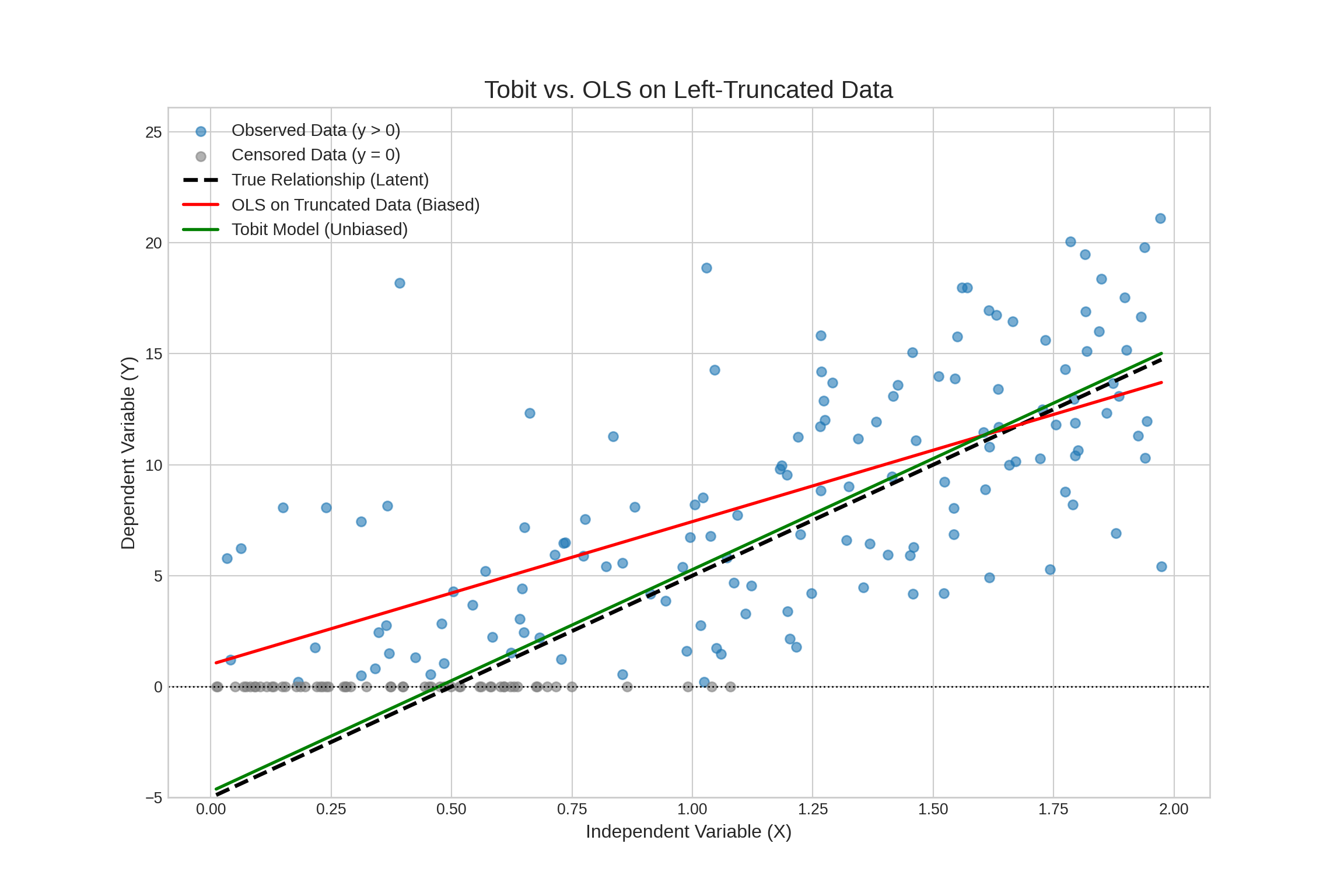
Why OLS Fails
- OLS on positives only: If we drop the zero-outcome observations, we induce selection bias.
- We are only looking at a group for whom the error term \(u_i\) was large enough to push \(y_i^*\) above zero.
- This means \(E[u_i | y_i > 0] \neq 0\), biasing the coefficients.
- OLS on all data (including zeros):
- The relationship between \(X\) and the observed \(y_i\) is non-linear. The conditional expectation \(E[y_i | X]\) is a complex function, not the simple linear form \(\beta_0 + \beta_1 X_1 + \dots\).
- OLS will incorrectly estimate the linear relationship, typically attenuating the coefficients towards zero.
Solution: Maximum Likelihood Estimation
We construct a likelihood function that accounts for the two types of observations:
- For an observation where \(y_i = 0\), its contribution to the likelihood is the probability that \(y_i^* \leq 0\).
- \(P(y_i^* \leq 0) = P(u_i \leq -(\beta_0 + \beta_1 X_{1i} + ...)) = \Phi(-\frac{\beta_0 + \beta_1 X_{1i} + ...}{\sigma})\)
- For an observation where \(y_i > 0\), its contribution is the probability density of observing that specific value of \(y_i\).
- This is the standard normal probability density function (PDF), evaluated at \(y_i\).
Hence, the likelihood is:
\[ \prod_{i=1}^N \Phi \left(-\frac{\beta_0 + \beta_1 X_{1i} + \dots}{\sigma}\right)^{I(Y_i = 0)} \cdot \phi \left(\frac{Y_j - [\beta_0 + \beta_1 X_{i1} + \dots]}{\sigma}\right)^{I(Y_i >0)} \]
MLE finds the parameter values (\(\beta_0, \beta_1, ..., \sigma\)) that maximize the joint probability (the product of these individual likelihoods) of observing our actual sample.
Interpretation
The estimated \(β\) coefficients measure the effect of an X-variable on the latent variable \(y^*\), not on the observed outcome \(y\).
For observations above the censoring point, the marginal effect is: \[ \frac{\partial E(y_i∣y_i>0,x_i)}{\partial x_j}=\beta_j \cdot Pr(y_i > 0| x_i) \]
- This means the effect of \(x_j\) on the observed \(y_i\) (for uncensored data) is attenuated by the probability of being uncensored.
Effect on the Expected Value of the Observed Variable (\(E[y_i]\)):
- The overall marginal effect (for both censored and uncensored observations) is: \(\frac{\partial E[y_i | x_i]}{x_j} =\beta_j \Phi(\frac{\beta_0 + \beta_1 x_{i1} + \dots}{\sigma})\)
- Hence, to find the effect on the observed outcome, one must calculate marginal effects, which are more complex.
Visualization
Summary
What did we do?
- Binary outcomes are everywhere.
- Standard OLS (the LPM) is a simple starting point but is flawed (out-of-range predictions, bad errors) in some ways, but good (interaction effects, integration with panel data) in others.
- Probit and Logit:
- These are the standard solutions. They are derived from a latent variable model and use a non-linear CDF to constrain predictions between 0 and 1.
- Maximum Likelihood Estimation (MLE):
- We looked at these models are estimated, MLE, which finds the parameters that make the observed data most probable.
- Interpretation:
- We found that raw coefficients are not marginal effects, we can use Average Marginal Effects (AMEs) to talk about changes in probability. In logit, we can use use Odds Ratios for Logit models for a multiplicative interpretation.
What did we do? (Cont.)
- Goodness-of-fit:
- We discussed various ways of evaluating binary outcome models, and discussed their pros and cons.
- Prediction:
- We talked about prediction on unseen data using different methods.
- Censored data:
- We talked about the Tobit model, which could deal with \([0, \infty]\) or otherwise censored data.
The End
![]()
Empirical Economics: Lecture 6 - Binary Outcome Data