| OLS | IV | |
|---|---|---|
| * p < 0.1, ** p < 0.05, *** p < 0.01 | ||
| Institutional Quality | 0.522*** | 0.944*** |
| (0.061) | (0.157) | |
| Constant | 4.660*** | 1.910* |
| (0.409) | (1.027) | |
| Num.Obs. | 64 | 64 |
| R2 Adj. | 0.533 | 0.469 |
Empirical Economics
Lecture 8: Instrumental Variables
Course Evaluations
Course Evaluations
We would really like you to take the time to fill out the course evaluation form. Your feedback is very important to us and helps us improve the course for future students.
You can fill it in anonymously on https://entry.caracal.uu.nl/44007 under “Course Evaluations” or scan the QR code:

Introduction
Course Overview
- Linear Model I
- Linear Model II
- Time Series and Prediction
- Panel Data I
- Panel Data II
- Binary Outcome Data
- Potential Outcomes and Difference-in-differences
- Instrumental Variables
\[ \newcommand{\Yobs}{Y^{\text{obs}}} \newcommand{\Ycf}{Y^{\text{cf}}} \newcommand{\E}{\mathbb{E}} \newcommand{\indep}{\perp \!\!\! \perp} \newcommand{\Cov}{\text{Cov}} \newcommand{\Var}{\text{Var}} \newcommand{\Prp}{\text{Pr}} \]
Causal Inference
The Goal of Causal Inference
Our fundamental goal is often to estimate the causal effect of a variable \(X\) on an outcome \(Y\).
Consider the simple linear model:
\[ Y_i = \beta_0 + \beta_1 X_i + u_i \]
We want our estimate of \(\beta_1\), which we call \(\hat{\beta}_1\), to be an unbiased and consistent estimate of the true causal effect.
For Ordinary Least Squares (OLS) to be unbiased, we need the regressor \(X\) to be uncorrelated with the error term \(\epsilon\): \(E[X_i u_i] = 0 \text{ or } Cov(X_i, u_i) = 0\)
- This is the assumption of exogeneity.
The Problem: Endogeneity
Endogeneity occurs when the exogeneity assumption is violated:
\[ Cov(X_i, u_i) \neq 0 \]
When \(X\) is endogenous, OLS is biased and inconsistent. Our \(\hat{\beta}_1\) does not converge to the true \(\beta_1\), even with infinite data.
Why does this happen?
- The error term \(u\) contains all other factors that determine \(Y\) but are not included in the model. If any of these omitted factors are also correlated with \(X\), we have a problem.
Sources of Endogeneity
Omitted Variable Bias (OVB)
- A variable \(W\) affects \(Y\) and is also correlated with \(X\), but \(W\) is not included in the model.
- Example: Effect of education (\(X\)) on wages (\(Y\)). Omitted “ability” (\(W\)) affects wages and is correlated with education.
- Direction of bias can be predicted.
- A variable \(W\) affects \(Y\) and is also correlated with \(X\), but \(W\) is not included in the model.
Simultaneity / Reverse Causality
- \(X\) causes \(Y\), but \(Y\) also causes \(X\).
- Example:Effect of police presence (\(X\)) on crime rates (\(Y\)). More police may reduce crime, but higher crime rates lead to more police being hired.
- Direction of bias unclear.
- \(X\) causes \(Y\), but \(Y\) also causes \(X\).
Measurement Error
- The variable \(X\) is measured with error.
- Example: Effect of household income (\(X\)) on consumption (\(Y\)). Income reported in surveys (\(X\)) is often an imperfect measure of true income.
- Attenuation bias toward 0.
- The variable \(X\) is measured with error.
Illustrating Omitted Variable Bias
Let the true model be:
\[ Y_i = \beta_0 + \beta_1 X_i + \beta_2 W_i + u_i \]
The omitted variable \(W_i\) is an unobserved variable (e.g., ability).
Suppose we estimate the simple model:
\[ Y_i = \alpha_0 + \alpha_1 X_i + \epsilon_i \quad (\text{where } \epsilon_i = \beta_2 W_i + u_i) \]
Then, the OLS estimate for \(\alpha_1\) will be:
\[ \hat{\alpha}_1 = \beta_1 + \beta_2 \cdot \frac{Cov(X_i, W_i)}{Var(X_i)} \]
The bias is \(\beta_2 \cdot \frac{Cov(X_i, W_i)}{Var(X_i)}\).
It is non-zero if \(W\) affects \(Y\) (\(\beta_2 \neq 0\)) and is correlated with \(X\) (\(Cov(X,W) \neq 0\)).
Omitted Variable Bias Example
Example: Wages, Education and Ability
Let \(Y_i\): The wage of an individual i, \(X_i\): The years of education, \(W_i\): The innate ability (e.g., intelligence, work ethic), which is impossible for the researcher to observe, \(u_i\): The random unobserved error term, representing other factors affecting wages (e.g., luck, measurement error). The true model for an individual’s wage is:
\[ \text{Wage}_i = \beta_0 + \beta_1 \text{Education}_i + \beta_2 \text{Ability}_i + u_i \]
Here, \(\beta_1\) is the true causal effect of an additional year of education on wages, holding ability constant. However, since we cannot observe ability (\(W_i\)), we are forced to estimate a simpler model:
\[ \text{Wage}_i = \alpha_0 + \alpha_1 \text{Education}_i + \epsilon_i \]
In this estimated model, the new error term \(\epsilon_i\) now contains both the original error and the effect of the omitted ability variable (\(\epsilon_i = \beta_2 \text{Ability}_i + u_i\)). The OLS estimate for the effect of education, \(\hat{\alpha}_1\), will be biased as shown by the formula:
\[ \hat{\alpha}_1 = \beta_1 + \beta_2 \cdot \frac{Cov(\text{Education}_i, \text{Ability}_i)}{Var(\text{Education}_i)} \]
The bias is the second term, \(\beta_2 \cdot \frac{Cov(\text{Education}_i, \text{Ability}_i)}{Var(\text{Education}_i)}\), and it is non-zero because:
- Ability affects wages (\(\beta_2 \neq 0\)): More able individuals are likely to earn higher wages, even with the same level of education.
- Education and ability are correlated (\(Cov(\text{Education}_i, \text{Ability}_i) \neq 0\)): Individuals with higher innate ability may find it easier to attain more years of education, creating a positive covariance.
Because both \(\beta_2\) and the covariance term are positive, our OLS estimate \(\hat{\alpha}_1\) will overestimate the true return to education (\(\beta_1\)). The model mistakenly attributes the wage premium from higher ability to the additional years of education.
Intuition for IV
Intuition for Instrumental Variables
If \(X\) is endogenous, we can’t use its correlation with \(Y\) to identify \(\beta_1\).
- Part of the correlation between \(X\) and \(Y\) is the causal effect we want (\(\beta_1\)).
- Another part is the “bad” correlation due to endogeneity (e.g., OVB).
The idea in IV is to find a third variable \(Z\), the instrument, that can isolate the “good” part of the variation in \(X\).
An instrument is a variable that is correlated with the endogenous regressor \(X\), but is not correlated with the error term \(\epsilon\).
- It creates “as-if random” variation in \(X\).
- It only affects \(Y\) its effect on \(X\).
Two Core IV Assumptions
For a variable \(Z\) to be a valid instrument for \(X\) in the model \(Y_i = \beta_0 + \beta_1 X_i + \epsilon_i\), it must satisfy two conditions:
- Relevance Condition (First Stage)
- The instrument \(Z\) must be correlated with the endogenous variable \(X\): \(Cov(Z_i, X_i) \neq 0\)
- This is testable from the data. We can regress \(X\) on \(Z\).
- Exclusion Restriction (Exogeneity)
- The instrument \(Z\) must be uncorrelated with the error term \(\epsilon\): \(Cov(Z_i, \epsilon_i) = 0\)
- This means \(Z\) affects \(Y\) only through its effect on \(X\).
- This is a theoretical assumption and is not testable. It requires deep institutional knowledge and a strong argument.
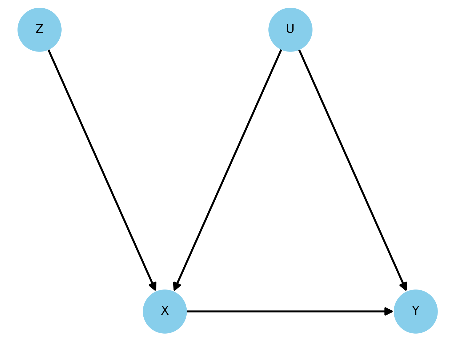
Visualize IV with a DAG
- In the graph below, \(U\) is an unobserved confounder.
- The path \(X \leftarrow U \rightarrow Y\) creates a spurious correlation between \(X\) and \(Y\). OLS is biased.
- The IV assumptions are:
- Relevance: The arrow \(Z \rightarrow X\).
- Exclusion Restriction: The of a direct arrow from \(Z\) to \(Y\) or from \(Z\) to \(U\).
IV and Potential Outcomes
Potential Outcomes (Reminder)
Let’s consider a binary treatment \(X_i \in \{0, 1\}\).
- \(Y_i(1)\): The potential outcome for individual \(i\) if they receive the treatment (\(X_i=1\)).
- \(Y_i(0)\): The potential outcome for individual \(i\) if they do not receive the treatment (\(X_i=0\)).
The individual causal effect is \(\tau_i = Y_i(1) - Y_i(0)\).
For each individual \(i\), we can only observe one of the two potential outcomes:
\[ Y_i^{\text{obs}} = X_i Y_i(1) + (1-X_i) Y_i(0) \]
We never observe \(Y_i(1)\) and \(Y_i(0)\) for the same person.
IV in a Potential Outcomes Framework
Now let’s introduce a binary instrument \(Z_i \in \{0, 1\}\).
- \(Z_i=1\): Individual \(i\) is “encouraged” to get treatment.
- \(Z_i=0\): Individual \(i\) is “not encouraged”.
We need to define potential outcomes for the treatment itself, based on the instrument:
- \(X_i(1)\): The treatment status of individual \(i\) if they are encouraged (\(Z_i=1\)).
- \(X_i(0)\): The treatment status of individual \(i\) if they are not encouraged (\(Z_i=0\)).
And we also have potential outcomes for \(Y\): \(Y_i(x)\), which depend on the treatment, which in turn depends on the instrument.
- \(Y_i (x)\) is shorthand for \(Y_i (X_i(Z_i))\).
Compliers, Always-Takers, Never-Takers
- Based on how an individual’s treatment status \(X_i\) responds to the instrument \(Z_i\), we can classify the population into four groups.
| Type | If \(Z_i=0\), \(X_i(0)\) is | If \(Z_i=1\), \(X_i(1)\) is | Description |
|---|---|---|---|
| Complier | 0 | 1 | (Does what they are encouraged to do) |
| Always-Taker | 1 | 1 | (Takes treatment regardless of encouragement) |
| Never-Taker | 0 | 0 | (Never takes treatment regardless) |
| Defier | 1 | 0 | (Does the opposite of encouragement) |
IV Assumptions in Potential Outcomes
- Like potential outcomes, we never know for sure which group an individual belongs to.
- The two core assumptions have precise meanings in this framework, plus we need two more.
Assumption: Treatment Assignment in IV
- Independence: \(Z_i \indep \{ Y_i(1), Y_i(0), X_i(1), X_i(0) \}\)
- The instrument is “as-if” randomly assigned. It’s independent of all potential outcomes and potential treatment decisions.
- Exclusion Restriction: \(Y_i(x, z) = Y_i(x) \quad \text{for all } x, z\)
- The instrument \(Z\) does not have a direct effect on the outcome \(Y\). It only works through \(X\).
- Relevance (First Stage): \(\E[X_i | Z_i=1] - \E[X_i | Z_i=0] \neq 0\)
- The instrument must affect the treatment status for some individuals. This means there must be some Compliers.
- Monotonicity: \(X_i(1) \geq X_i(0) \quad \text{for all } i\)
- The instrument encourages (or discourages) everyone weakly in the same direction. This assumption rules out the existence of Defiers
IV Estimator
With these four assumptions, IV does not estimate the Average Treatment Effect (\(ATE = E[Y_i(1) - Y_i(0)]\)) for the whole population.
Instead, IV estimates the Local Average Treatment Effect (LATE)
Theorem: LATE (Imbens & Angrist, 1994)
\[ \beta_{IV} = E[Y_i(1) - Y_i(0) \mid X_i(1) > X_i(0)] \]
This is the average treatment effect only for the subpopulation of compliers.
This is a crucial insight: The causal effect we get from IV is specific to the group of people who are induced into treatment by the instrument. It may not generalize to Always-Takers or Never-Takers.
Wald Estimator
The Wald Estimator
The simplest IV estimator is the Wald estimator, used when both the instrument \(Z\) and the treatment \(X\) are binary.
\[ \hat{\beta}_{\text{Wald}} = \frac{E[Y | Z=1] - E[Y | Z=0]}{E[X | Z=1] - E[X | Z=0]} \]
Interpretation:
- Numerator: The “Reduced Form” effect. How much does the outcome change when the instrument is switched on?
- Called the Intent-to-Treat (ITT) effect
- Denominator: The “First Stage” effect. How much does the treatment take-up change when the instrument is switched on?
- Called the share of compliers.
- Numerator: The “Reduced Form” effect. How much does the outcome change when the instrument is switched on?
The Wald estimator is simply the sample-analogue of this formula.
LATE Theorem (Heuristic)
Why does the Wald formula gives us the LATE?
The numerator is \(E[Y | Z=1] - E[Y | Z=0]\)
This difference in outcomes is only driven by the Compliers switching from \(X=0\) to \(X=1\).
For everyone else (Always/Never-Takers), their treatment status doesn’t change. So the numerator can be rewritten as:
\[ \text{Numerator} = \Pr(\text{Complier}) \cdot \E[Y(1) - Y(0) \mid \text{Complier}]=\Pr(\text{Complier})\cdot LATE. \]
The denominator is \(\E[X | Z=1] - \E[X | Z=0] = \Pr(\text{Complier})\)
Together:
\[ \hat{\beta}_{\text{Wald}} = \frac{\Pr(\text{Complier}) \cdot \text{LATE}}{\Pr(\text{Complier})} = \text{LATE} \]
Proof of LATE Theorem
Let’s prove that the Wald estimator identifies the LATE under the four key IV assumptions (Independence, Exclusion, Relevance, Monotonicity).
\[ \text{Wald} = \frac{\E[Y | Z=1] - \E[Y | Z=0]}{\E[X | Z=1] - \E[X | Z=0]} \]
We will show that \(\E[X | Z=1] - \E[X | Z=0] = \Prp(\text{Complier})\).
\[ \begin{align*} \E[X | Z=z] &= \E[X_i(z) | Z=z] && \text{(Def. of observed X)} \\ &= \E[X_i(z)] && \text{(by Independence assumption)} \end{align*} \]
Proof of LATE Theorem (Cont.)
So the denominator is \(\E[X_i(1)] - \E[X_i(0)]\). Let’s expand this using the Law of Total Expectation over the population types (C=Complier, A=Always-Taker, N=Never-Taker). We assume Monotonicity, so there are no Defiers.
\[ \begin{align*} \E[X_i(1)] &= \E[X_i(1)|C]\Prp(C) + \E[X_i(1)|A]\Prp(A) + \E[X_i(1)|N]\Prp(N) \\ &= (1)\Prp(C) + (1)\Prp(A) + (0)\Prp(N) = \Prp(C) + \Prp(A) \\ \E[X_i(0)] &= \E[X_i(0)|C]\Prp(C) + \E[X_i(0)|A]\Prp(A) + \E[X_i(0)|N]\Prp(N) \\ &= (0)\Prp(C) + (1)\Prp(A) + (0)\Prp(N) = \Prp(A) \end{align*} \]
Therefore, the denominator is:
\[ (\Prp(C) + \Prp(A)) - \Prp(A) = \Prp(C) \]
Proof of LATE Theorem (Cont.)
The numerator can be interpreted as the Intent-to-Treat for Compliers.
The numerator is \(\E[Y | Z=1] - \E[Y | Z=0]\). Again, we use Independence to state that:
\[ \E[Y | Z = z] = \E[Y_i(X_i(z)) | Z = z] = \E[Y_i(X_i(z))] \]
Dissecting these two terms gives:
\[ \begin{align*} \E[Y_i(X_i(1))] &= \E[Y_i(X_i(1))|C]\Prp(C) + \E[Y_i(X_i(1))|A]\Prp(A) + \E[Y_i(X_i(1))|N]\Prp(N) \\ &= \E[Y_i(1)|C]\Prp(C) + \E[Y_i(1)|A]\Prp(A) + \E[Y_i(0)|N]\Prp(N) \\ \E[Y_i(X_i(0))] &= \E[Y_i(X_i(0))|C]\Prp(C) + \E[Y_i(X_i(0))|A]\Prp(A) + \E[Y_i(X_i(0))|N]\Prp(N) \\ &= \E[Y_i(0)|C]\Prp(C) + \E[Y_i(1)|A]\Prp(A) + \E[Y_i(0)|N]\Prp(N) \end{align*} \]
Proof of LATE Theorem (Cont.)
Now, we take the difference.
- Notice the terms for Always-Takers and Never-Takers are identical and will cancel out:
\[ \begin{align*} \text{Numerator} &= \left( \E[Y_i(1)|C]\Prp(C) + \dots \right) - \left( \E[Y_i(0)|C]\Prp(C) + \dots \right) \\ &= \E[Y_i(1)|C]\Prp(C) - \E[Y_i(0)|C]\Prp(C) \\ &= \Prp(C) \cdot \left( \E[Y_i(1)|C] - \E[Y_i(0)|C] \right) \\ &= \Prp(\text{Complier}) \cdot \E[Y_i(1) - Y_i(0) | \text{Complier}] \\ &= \Prp(\text{Complier}) \cdot \text{LATE} \end{align*} \]
The Exclusion Restriction is implicitly used because \(Y\) only depends on \(X\), not \(Z\).
Putting It All Together
There fore, we have shown:
\[ \textbf{Numerator} = \Prp (\text{Complier}) \times \text{LATE} \\ \textbf{Denominator} = \Prp (\text{Complier}) \]
And the Wald estimator is:
\[ \hat{\beta}_{\text{Wald}} = \frac{\E[Y | Z=1] - \E[Y | Z=0]}{\E[X | Z=1] - \E[X | Z=0]} = \frac{\Prp(\text{Complier}) \times \text{LATE}}{\Prp(\text{Complier})} = \text{LATE} \]
This shows that the simple ratio of the reduced form effect to the first-stage effect precisely isolates the average causal effect for the specific subpopulation whose treatment status is actually manipulated by the instrument.
Estimating Complier Shares
- Being a complier, never-taker or always-taker is a latent characteristic of an individual \(i\).
- Given our assumptions of monotonicity and no defiers, if we observe \(X_i (1) = 1\) or \(X_i (0)=0\), we will never know whether \(i\) is a complier or an always taker (never taker).
- However, if we observe \(X(0)=1\) (\(X(1)=0\)), we know an individual is an always-taker (never-taker).
- You can infer the proportions of compliers, always takers and never-takers in the population as follows:
- Since \(Z \indep X\), proportions are preserved by conditioning on the instrument.
- Group that was not encouraged: \(E[X|Z=0] = P(A)\).
- Group that was encouraged: \(E[X|Z=1] = P(A) + P(C)\)
- Collective exhaustedness: \(P(A) + P(C) + P(N)=1\)
- This is why, even though we can’t identify every single individual’s type, we can identify the proportions of each type at the population level by looking at the sample averages.
Example
Example: Acemoglu, Johnson and Robinson (2000)
Example: AJR (2001)
- A central question in development economics is whether strong institutions (secure property rights, rule of law) are a fundamental cause of economic growth.
\(Y\): Economic growth (Log GDP per capita)
\(X\): Institutional quality (average protection against expropriation risk)
\(Z\): Log of Settler Mortality Rates
Endogeneity: A simple OLS regression of Log GDP per capita on a measure of Institutional Quality is likely biased.
- Reverse Causality: Rich countries may be able to afford better institutions.
- Omitted Variable Bias: Other factors, like geography or culture, could determine both institutional and economic outcomes.
Example: AJR (2001)
Their theory: Settler Mortality \(\rightarrow\) European Settlements \(\rightarrow\) Early Institutions \(\rightarrow\) Current Institutions \(\rightarrow\) Current Economic Performance
- Different Colonization Strategies: Europeans established different types of colonies.
- “Neo-Europes” (Inclusive Institutions): In places with low settler mortality (e.g., USA, Australia), Europeans settled in large numbers and replicated institutions that protected private property and constrained government power.
- “Extractive States”: In places with high settler mortality due to diseases like malaria and yellow fever (e.g., Congo, Nigeria), Europeans established authoritarian and extractive institutions with the sole purpose of transferring resources back to the colonizer.
Persistence of Institutions: these initial institutions, whether inclusive or extractive, have persisted to the present day.
Example: AJR (2001)
- Main Result: The 2SLS estimates show a large and statistically significant effect of institutions on economic development. The results suggest that differences in institutions explain the majority of the income disparity across former colonies.
General IV Estimator
General IV Estimator
Let’s return to our linear model \(Y_i = \beta_0 + \beta_1 X_i + u_i\) where \(\Cov(X_i, u_i) \neq 0\). We have an instrument \(Z\) such that \(\Cov(Z_i, X_i) \neq 0\) and \(\Cov(Z_i, u_i) = 0\).
The IV estimator for \(\beta_1\) is given by:
\[ \hat{\beta}_1^{\text{IV}} = \frac{\Cov(Z, Y)}{\Cov(Z, X)} \]
Notice the similarity to the Wald estimator. The numerator is the covariance of the instrument and outcome (reduced form), and the denominator is the covariance of the instrument and the endogenous variable (first stage).
Analogy to OLS Estimator
This formula is very instructive. Let’s compare it to the OLS estimator in a simple regression.
OLS Estimator:\(\hat{\beta}_1^{\text{OLS}} = \frac{\Cov(X, Y)}{\Cov(X, X)} = \frac{\Cov(X, Y)}{\Var(X)}\).
- OLS uses the full covariance of \(X\) and \(Y\). If \(X\) is endogenous, this covariance is “contaminated.”
IV Estimator: \(\hat{\beta}_1^{\text{IV}} = \frac{\Cov(Z, Y)}{\Cov(Z, X)}\) IV replaces the “bad” variation in \(X\) with the “good” variation in \(Z\).
- It uses only the part of the variation in \(X\) that is induced by the exogenous instrument \(Z\).
- It then scales the relationship between \(Z\) and \(Y\) by the relationship between \(Z\) and \(X\).
General Case: Two-Stage Least Squares (2SLS)
What if we have multiple instruments or other exogenous control variables (\(W\))?
- We use a procedure called Two-Stage Least Squares (2SLS).
Let the structural model be \(Y_i = \beta_0 + \beta_1 X_i + \gamma' W_i + u_i\) (\(X_i\) is endogenous, \(W_i\) are exogenous controls).
Let the instruments be \(Z_1, Z_2, ..., Z_k\).
The 2SLS procedure works in two steps…
2SLS: The First Stage
First Stage Regression: Regress the endogenous variable \(X\) on all the instruments \(Z\) and all other exogenous controls \(W\).
\[ X_i = \pi_0 + \pi_1 Z_{1i} + ... + \pi_k Z_{ki} + \delta' W_i + \nu_i \]
From this regression, we obtain the for \(X\), which we call \(\hat{X}_i\).
\[ \hat{X}_i = \hat{\pi}_0 + \hat{\pi}_1 Z_{1i} + ... + \hat{\pi}_k Z_{ki} + \hat{\delta}' W_i \]
This \(\hat{X}_i\) is the part of the variation in \(X\) that is explained by our exogenous variables.
- By construction, \(\hat{X}_i\) is uncorrelated with the structural error \(\epsilon_i\) (as long as our instruments are valid!).
2SLS: The Second Stage
Second Stage Regression: Regress the outcome variable \(Y\) on the endogenous variable \(\hat{X}\) and the other exogenous controls \(W\).1
\[ Y_i = \beta_0 + \beta_1 \hat{X}_i + \gamma' W_i + \zeta_i \]
The coefficient \(\hat{\beta}_1\) from this second stage regression is our 2SLS estimate.
Since we used \(\hat{X}_i\) instead of \(X_i\), we have purged the endogeneity, and our estimate for \(\beta_1\) is now consistent.
Finding Good Instruments
The credibility of any IV analysis rests entirely on the quality of the instrument.
A good instrument must be both relevant and valid (exogenous).
The exclusion restriction is a very strong assumption. You must provide a convincing story for why your instrument \(Z\) could not possibly affect \(Y\) except through its effect on \(X\).
Often, instruments come from:
- Natural or quasi-random experiments (e.g., policy changes, lotteries).
- Institutional details or rules.
- Geographic or historical quirks.
The Problem of Weak Instruments
What happens if the relevance condition is only barely met? In other words, if \(\Cov(Z,X)\) is very close to zero?
If an instrument is weak, even a tiny violation of the exclusion restriction (a tiny \(\Cov(Z, \epsilon)\)) can lead to a very large bias in the IV estimate.
\[ \text{Bias}(\hat{\beta}_{IV}) \approx \frac{\Cov(Z, \epsilon)}{\Cov(Z, X)} \]
A small denominator leads to a large bias! Furthermore, the variance of the IV estimator will be very large.
Testing for Weak Instruments
We can and should test for instrument relevance.
- This is a test on the regression:
\[ X_i = \pi_0 + \pi_1 Z_{1i} + ... + \pi_k Z_{ki} + (\text{controls}) + \nu_i \]
We perform an F-test on the joint significance of all instruments:
\[ H_0: \pi_1 = \pi_2 = ... = \pi_k = 0 \]
A first-stage F-statistic greater than 10 is often used as a benchmark to indicate that instruments are not weak (Stock, Wright, & Yogo, 2002). \(F < 10\) is a serious red flag.
- You should always report the first-stage F-statistic in any IV analysis.
Testing the Exclusion Restriction
- The exclusion restriction, \(\Cov(Z, \epsilon)=0\), is the bedrock of IV and is fundamentally untestable.
- Its validity is based on economic theory, institutional knowledge, and careful reasoning.
- However, if you have more instruments than endogenous variables (the “overidentified” case), you can perform a partial test (Sargan-Hansen test).
- Intuition: If all instruments are valid, they should all point to the same estimate of \(\beta_1\). The test checks if the different instruments produce statistically different estimates.
- A rejection of the null hypothesis suggests that at least one of your instruments is not valid (i.e., it is correlated with the error term).
- This test requires you to believe that at least one instrument is valid to test the validity of the “extra” ones.
Classic IV Example: Angrist & Krueger (1991)
Research Question: What is the causal effect of an additional year of schooling on wages?
Outcome (\(Y\)): Log weekly wages.
- Endogenous Variable (\(X\)): Years of schooling.
- Endogeneity Problem: Ability is an omitted variable.
- More able individuals tend to get more schooling and earn higher wages, biasing the OLS estimate upwards.
The Instrument (\(Z\)): Quarter of Birth.
Angrist & Krueger (1991): The Instrument
Why is Quarter of Birth a valid instrument?
Institutional Detail: In the US, compulsory schooling laws required students to attend school until they turned 16 or 17.
- Students born early in the year (e.g., Jan, Feb) start school at an older age. They turn 16 earlier in their school career and can legally drop out with slightly less education.
- Students born late in the year (e.g., Oct, Nov) are younger when they start school. They are forced by the law to stay in school longer to reach their 16th birthday, resulting in slightly more education on average.
IV Assumptions:
- Relevance: Is quarter of birth correlated with years of schooling? Yes, the data showed a small but statistically significant relationship.
- Exclusion restriction: Is it plausible that quarter of birth has no direct effect on wages, other than through its effect on schooling? It’s hard to think of a reason why birth month would directly influence adult earnings, other than this institutional reason.
Angrist & Krueger (1991): Results
OLS Result: Found that an extra year of school was associated with about a 7.5% increase in wages.
- Likely an overestimate due to ability bias.
- Why is this an overestimate? Think about the OVB formula and the correlation between \(X\) and \(Z\)
2SLS Result: Using quarter of birth as an instrument, they found a very similar return to schooling, also around 7.5%.
Interpretation (LATE):
- This IV estimate is the Local Average Treatment Effect.
- It represents the return to schooling for the compliers: those individuals who were induced to stay in school for an extra bit of time because of compulsory schooling laws.
- These are likely people on the margin of dropping out of high school. The result may not apply to the returns to getting a college degree.
Other Example: Demand Estimation
Let’s say we want to estimate the price elasticity of demand for avocados.
The starting point is a so-called structural model.
- Demand Curve: We want to estimate this equation. \(\alpha_1\) is our parameter of interest (the elasticity). \[ Q_i^d = \alpha_0 + \alpha_1 P_i + u_i \]
- \(u_i\) represents unobserved demand shocks (e.g., a new health trend, a guacamole festival).
- Supply Curve: The market also has a supply curve. \[ Q_i^s = \beta_0 + \beta_1 P_i + v_i \]
- \(v_i\) represents unobserved supply shocks (e.g., a localized pest).
- Demand Curve: We want to estimate this equation. \(\alpha_1\) is our parameter of interest (the elasticity). \[ Q_i^d = \alpha_0 + \alpha_1 P_i + u_i \]
The Endogeneity Issue
In market equilibrium, \(Q_i^d = Q_i^s = Q_i\), and the price \(P_i\) adjusts to make this happen. This means price \(P_i\) is determined by both supply and demand factors.
If there is a positive demand shock (\(u_i > 0\)), the demand curve shifts right. This leads to a higher equilibrium price and a higher quantity.
Therefore, \(P_i\) is positively correlated with the demand error term \(u_i\).
This violates the core OLS assumption that regressors are uncorrelated with the error term: \(Cov(P_i, u_i) \neq 0\).
Running OLS of \(Q\) on \(P\) will give a biased estimate of \(\alpha_1\).
The Solution: IV
- We need a variable, let’s call it \(Z\), that provides an exogenous source of variation in price. This variable is our Instrument.
Example: Good Instrument
Let \(Z_i\) be a measure of growing conditions (e.g., rainfall in avocado-growing regions). Good weather increases supply.
The Updated Structural Model
Demand Curve (Unchanged): Weather doesn’t directly affect how many avocados a person wants to buy at a given price. \[ Q^d_i = \alpha_0 + \alpha_1 P_i + u_i \]
Supply Curve (with Instrument): Weather directly affects the quantity supplied. \[ Q^s_i = \beta_0 + \beta_1 P_i + \delta Z_i + v_i \]
The Two IV Conditions (in this context)
Remember that an instrument needs to satisfy two key conditions:
- Relevance: The instrument must affect the endogenous variable. Good weather must actually change the price of avocados.
- Algebraically: \(\delta \neq 0\), which implies \(Cov(Z_i, P_i) \neq 0\).
- Exclusion Restriction: The instrument must be uncorrelated with the error term in the primary equation (demand). Good weather doesn’t directly cause a craving for avocados.
- Algebraically: \(Cov(Z_i, u_i) = 0\). This is the crucial identifying assumption.
- Relevance: The instrument must affect the endogenous variable. Good weather must actually change the price of avocados.
Identification: The Algebra of IV
How do we use our instrument \(Z\) and the exclusion restriction to find \(\alpha_1\)?
Our goal is to estimate \(\alpha_1\) from the demand equation: \[ Q^d_i = \alpha_0 + \alpha_1 P_i + u_i \]
The problem is that \(Cov(P_i, u_i) \neq 0\). But we have assumed \(Cov(Z_i, u_i) = 0\). Let’s use that!
Step 1: Take the covariance of the demand equation with our instrument \(Z_i\).
\[ Cov(Z_i, Q^d_i) = Cov(Z_i, \alpha_0 + \alpha_1 P_i + u_i) \]
Step 2: Use the properties of covariance to expand the right side.
\[ Cov(Z_i, Q^d_i) = Cov(Z_i, \alpha_0) + Cov(Z_i, \alpha_1 P_i) + Cov(Z_i, u_i) \]
Identification: The Algebra of IV (Cont.)
Step 3: Simplify.
- \(Cov(Z_i, \alpha_0) = 0\) (covariance with a constant is zero).
- \(Cov(Z_i, \alpha_1 P_i) = \alpha_1 Cov(Z_i, P_i)\) (constants can be pulled out).
- \(Cov(Z_i, u_i) = 0\) (this is our crucial Exclusion Restriction assumption!).
Step 4: See what’s left. \[ Cov(Z_i, Q_i) = \alpha_1 Cov(Z_i, P_i) \]
Step 5: Solve for our parameter of interest, \(\alpha_1\). \[ \alpha_1 = \frac{Cov(Z_i, Q^d_i)}{Cov(Z_i, P_i)} \]
This is the instrumental variables estimator for \(\alpha_1\).
The Link to Reduced Form & First Stage
The expression \(\frac{Cov(Z_i, Q_i)}{Cov(Z_i, P_i)}\) has a beautiful and intuitive interpretation. Let’s look at two simple regressions.
- The First Stage: How does our instrument (\(Z\)) affect our endogenous variable (\(P\))? \[ P_i = \pi_{p0} + \pi_{p1} Z_i + u_p \]
- The OLS estimate of \(\pi_{p1}\) is: \(\hat{\pi}_{p1} = \frac{Cov(Z_i, P_i)}{Var(Z_i)}\).
- This tells us how much price changes for a one-unit change in weather.
- The Reduced Form: How does our instrument (\(Z\)) affect our final outcome (\(Q\))? \[ Q_i = \pi_{q0} + \pi_{q1} Z_i + u_q \]
- The OLS estimate of \(\pi_{q1}\) is: \(\hat{\pi}_{q1} = \frac{Cov(Z_i, Q_i)}{Var(Z_i)}\).
- This tells us how much quantity changes for a one-unit change in weather.
- The First Stage: How does our instrument (\(Z\)) affect our endogenous variable (\(P\))? \[ P_i = \pi_{p0} + \pi_{p1} Z_i + u_p \]
Ratio of RF and FS
Let’s look at the ratio of these two coefficients:
\[ \frac{\hat{\pi}_{q1}}{\hat{\pi}_{p1}} = \frac{ \frac{Cov(Z_i, Q_i)}{Var(Z_i)} }{ \frac{Cov(Z_i, P_i)}{Var(Z_i)} } = \frac{Cov(Z_i, Q_i)}{Cov(Z_i, P_i)} \]
This is exactly our IV estimator!
\[ \hat{\alpha}_{1, IV} = \frac{\text{Reduced Form Effect}}{\text{First Stage Effect}} = \frac{\text{Effect of Z on Q}}{\text{Effect of Z on P}} \]
The structural parameter \(\alpha_1\) is identified because it can be expressed as the ratio of two estimable parameters from simple regressions. We have used the exogenous variation from the instrument to isolate the causal effect of price on quantity demanded.
IV in Software
IV in R/Python/Stata
- All standard software packages support implementation of IV regression.
Code
# 1. Install and load necessary packages
#install.packages(c("fixest", "AER"))
library(fixest)
library(AER)

# 2. Estimate the IV model
# The formula is read as: y regressed on controls,
# with x being instrumented by z.
iv_model_r <- feols(y ~ controls | x ~ z, data = df)

# 3. Display the results
summary(iv_model_r)
Code
# 1. Install necessary packages
# !pip install pyfixest pandas statsmodels

# 2. Import libraries and load data
import numpy as np
import pandas as pd
from pyfixest.estimation import feols
import statsmodels.api as sm # Used to easily load the R dataset

# 3. Estimate the IV model using the R-style formula
# The formula is identical to the one used in R
iv_model_py = feols('y ~ controls | x ~ z', data=df)

# 4. Display the results
iv_model_py.summary()
Code
* 1. Load the data
use "dataset.csv", clear

* 2. Estimate the IV model
* Syntax: ivregress 2sls depvar [exog_vars] (endog_var = instrument_vars)
ivregress 2sls y controls (x = z)

* To get robust standard errors, which is often the default in R/Python packages
ivregress 2sls y controls (x = z), robust
Testing for Relevance
- The standard test for instrument relevance is the first-stage F-statistic. This test checks if the instruments are jointly significant predictors of the endogenous variable. A common rule of thumb is that an F-statistic greater than 10 suggests the instruments are sufficiently strong.
Code
# 1. Estimate the IV model
iv_model_r <- feols(y ~ controls | x ~ z, data = df)

# 2. Use the fitstat() function to extract various versions of first stage F statistics:
fitstat(iv_model_r, "cd") # For the Craig-Donald F Stat.
fitstat(iv_model_r, "kp") # For the Kleibergen-Paap F Stat.
fitstat(iv_model_r, "ivf") # For the standard F Stat.
Code
from pyfixest.estimation import feols
import statsmodels.api as sm # Used to easily load the R dataset

# 1. Estimate the IV model using the R-style formula
iv_model_py = feols('y ~ controls | x ~ z', data=df)

# 2. Look at F stat
# You can access the F-Statistic of the first stage via the _f_stat_1st_stage attribute:
iv_model_py._f_stat_1st_stage

# 3. Via the IV_Diag method, you can compute additional IV Diagnostics, as the effective F-statistic following Olea & Pflueger (2013):
iv_model_py.IV_Diag()
iv_model_py._eff_FSummary
What did we do?
Problem: Endogeneity (\(\Cov(X, \epsilon) \neq 0\)) makes OLS biased and inconsistent for estimating causal effects.
- Solution: A valid Instrumental Variable (\(Z\)) is:
- Relevant: Correlated with \(X\).
- Exogenous: Uncorrelated with the error term \(\epsilon\) (the Exclusion Restriction).
- Solution: A valid Instrumental Variable (\(Z\)) is:
Interpretation: IV estimates the Local Average Treatment Effect (LATE) - the causal effect for the subpopulation of “compliers” whose behavior is changed by the instrument.
Estimation: Use the Wald estimator for simple cases, and Two-Stage Least Squares (2SLS) for the general case.
In Practice: Finding a valid instrument is the hardest part. Always check for weak instruments (First-stage F-statistic) and be prepared to defend your exclusion restriction.
The End
![]()
Empirical Economics: Lecture 8 - Instrumental Variables