Empirical Economics
Prerequisite Knowledge - Probability and Statistics
Course Overview
- Linear Model I
- Linear Model II
- Time Series and Prediction
- Panel Data I
- Panel Data II
- Binary Outcome Data
- Potential Outcomes and Difference-in-differences
- Instrumental Variables
What do we need to learn?
- How do we model the processes that might have generated our data?
- Probability
- How do we summarize and describe data, and try to uncover what process may have generated it?
- Statistics
- How do we uncover patterns between variables?
- The linear model and further econometrics
Probability
Experiments, Outcomes, and Sample Spaces
- Experiment: A process or action whose result is uncertain.
- Example: Rolling a six-sided die.
- Example: Surveying a household to ask about their income.
- Example: Observing next year’s GDP growth rate.
- Outcome (\(X\)): A single possible result of an experiment.
- Example: The die shows a \(4\).
- Example: The household’s income is \(52,000\).
- Example: GDP growth is \(2.3%\).
- Sample Space (\(S\)): The set of all possible outcomes of an experiment.
- Example (Die Roll): \(S = {1, 2, 3, 4, 5, 6}\)
- Example (Household Income): \(S \in [0, \infty]\)
Events
Event: any collection of outcomes (including individual outcomes, the entire sample space, and the null set)
Using the die roll example where \(S = {1, 2, 3, 4, 5, 6}\), and each outcome is equally likely:
Example
- Event A: The outcome is an even number.
- \(A = {2, 4, 6}\)
- The probability of Event A is \(P(A) = \frac{3}{6} = 0.5\)
- Event B: The outcome is greater than 4.
- \(B = {5, 6}\)
- The probability of Event B is \(P(B) = \frac{2}{6} \approx 0.33\)
Intersections and Unions
The union of two events \(A\) and \(B\), denoted \(A \cup B\) is the event that either \(A\) occurs, \(B\) occurs, or both occur.
\[ P(A \cup B) = P(A) + P(B) - P(A \cap B) \]
- This accounts for the overlap between \(A\) and \(B\).
The intersection of two events \(A\) and \(B\), denoted \(P(A \cap B)\), is the event that both \(A\) and \(B\) occur simultaneously.
Example
Continuing the dice example:
The intersection of A and B (\(A \cap B\)): The outcome is even AND greater than 4.
- \(A \cap B = {6}\)
- \(P(A \cap B) = 1 / 6\)
What is the probability of the union of A and B?
- \(A \cup B\): The outcome is even OR greater than 4
Conditional Probability
- Conditional Probability is the probability of an event occurring, given that another event has already occurred.
- The probability of event A occurring given that event B has occurred is written as \(P(A|B)\).
Definition: Conditional Probability
\[P(A|B) = \frac{P(A \cap B)}{P(B)}\]
- Intuition: We are restricting our sample space. We know \(B\) happened, so the “universe” of possible outcomes is now just \(B\).
- Within that new universe, we want to know the chance that \(A\) also happens.
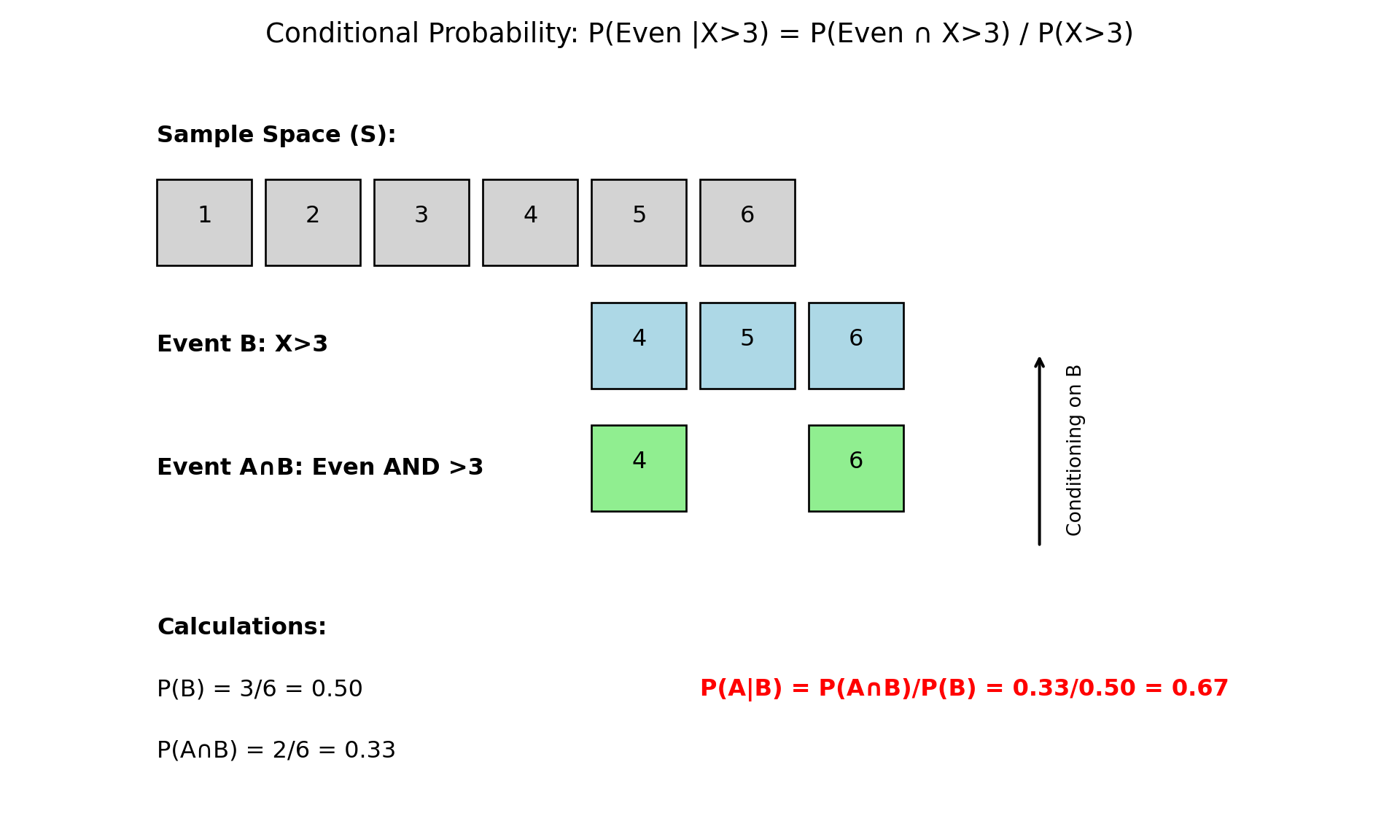
Conditional Probability: Example
- Let’s use our die roll example again:
Example
\(S = {1, 2, 3, 4, 5, 6}\), \(A = \{\text{Outcome is an even number}\} = \{2, 4, 6\}\), \(B = \{\text{Outcome is greater than 3}\} = \{4, 5, 6\}\)
Question: What is the probability that the number is even, given that we know it is greater than 3? We want to find \(P(A|B)\).
- Find \(P(B)\): The probability of rolling a number greater than 3 is \(P(B) = 3/6\).
- Find \(P(A \cap B)\): The probability of rolling a number that is even AND greater than 4 is \(P({5, 6}) = 2/6\).
- Apply the formula: \[P(A|B) = \frac{P(A \cap B)}{P(B)} = \frac{2/6}{3/6} = \frac{2}{3} \approx 0.67\]
Conditional Probability (Graphically)
- Intuition Check: If we know the outcome is in \(B = {4, 5, 6}\), there are only two possibilities. Of these, only two (\(4, 6\)) are even. So the probability is \(2/3\).
Random Variables, Expected Value, Variance
Random Variables
Random Variable (RV): A variable whose value is a numerical outcome of an experiment. We use capital letters (e.g., \(X\), \(Y\)) to denote a random variable.
There are two main types of random variables:
Discrete Random Variable: A variable that can only take on a finite or countably infinite number of distinct values.
Example
- The number of heads in three coin flips (\(X\) can be 0, 1, 2, 3).
- The number of defaults in a portfolio of 100 loans (\(X\) can be 0, 1, …, 100).
Random Variables
- Continuous Random Variable: A variable that can take on any value within a given range.
Example
- The exact price of a stock tomorrow.
- The annual percentage growth in GDP (\(Y\) could be 2.1%, 2.11%, 2.113%…).
Probability Mass Function
- For a discrete random variable \(X\), the Probability Mass Function (PMF) gives the probability that \(X\) is exactly equal to some value \(x\).
Definition: Probability Mass Function
\[ f(x) = P(X = x) \]
- A PMF has two key properties:
- \(0 \leq f(x) \leq 1\) for all \(x\).
- \(\sum f(x) = 1\) (The sum of probabilities over all possible values is 1).
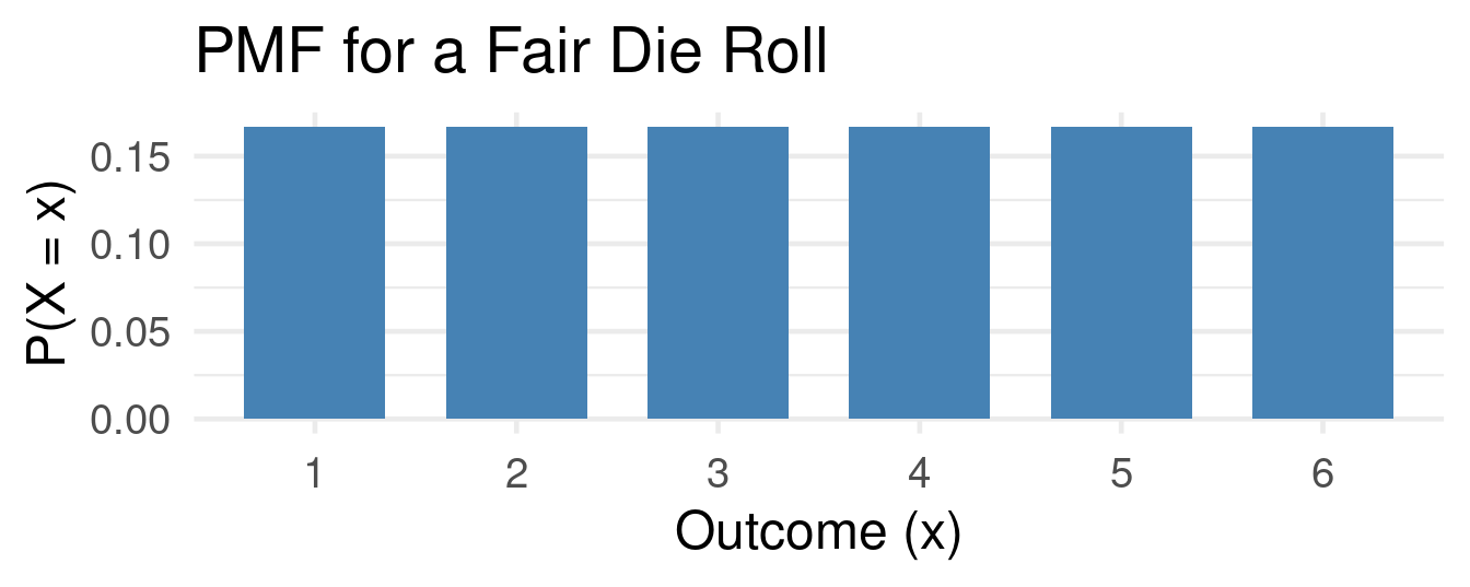
PMF Example
Example Probability Mass Function
Let \(X\) be the outcome of a fair die roll. The PMF is: \(f(1) = 1/6\), \(f(2) = 1/6\), …, \(f(6) = 1/6\).
Expected Value
- The Expected Value of a discrete random variable \(X\), denoted \(E[X]\) or \(\mu\), is the long-run average value of the variable.
- It’s a weighted average of the possible outcomes, where the weights are the probabilities.
Definition: Expected Value
\[ E[X] = \mu = \sum_x x \cdot P(X=x) \]
Example: Expected value of a fair die roll
\(E[X] = (1 \times {1 \over 6}) + (2 \times {1 \over 6}) + (3 \times {1 \over 6}) + (4 \times {1 \over 6}) + (5 \times {1 \over 6}) + (6 \times {1 \over 6})\) \(\hspace{2.5em} = (1+2+3+4+5+6) / 6 = 21 / 6 = 3.5\)
Note: The expected value doesn’t have to be a possible outcome!
Variance and Standard Deviation
- Variance, denoted \(Var(X)\) or \(\sigma^2\), measures the spread or dispersion of a random variable around its mean. A larger variance means the outcomes are more spread out.
Definition: Variance
\[ Var(X) = \sigma^2 = E[(X - \mu)^2] = \sum_x (x-\mu)^2 \cdot P(X=x) \]
- Standard Deviation, \(SD(X)\) or \(\sigma\), is the square root of the variance. It’s often easier to interpret because it’s in the same units as the random variable itself.
\[SD(X) = \sigma = \sqrt{Var(X)}\]
Example: The Bernoulli Distribution
Example: Bernoulli
The Bernoulli distribution is a fundamental discrete distribution for any experiment with two outcomes, typically labeled “success” (1) and “failure” (0).
Let \(X\) be a Bernoulli random variable where \(P(X=1) = p\) and \(P(X=0) = 1-p\). A Bernoulli distribution models binary outcomes like employed/unemployed, default/no-default, buy/don’t-buy.
Expected Value: \(E[X] = (1 \times p) + (0 \times (1-p)) = p\)
Variance: \[\begin{align*} Var(X) &= (1-p)^2 \times p + (0-p)^2 \times (1-p) \\ \qquad &= (1-p)^2 \times p + p^2 \times (1-p) \\ \qquad &= p(1-p) \times [(1-p) + p] = p(1-p) \end{align*}\]
Independence
Independence
Two events A and B are independent if:
\[ P(A \cap B) = P(A) \times P(B) \]
or equivalently:
\[ P(A|B) = P(A) \]
- Independence means one event doesn’t affect the other’s probability
- Mutually exclusive \(\neq\) independent (actually, mutually exclusive events with positive probability are dependent)
- Independence can extend to more than two events
Independence: Example
Example: Coin Flip
- Consider flipping a fair coin twice:
- Let A = “First toss is Heads”, \(P(A) = \frac{1}{2}\)
- Let B = “Second toss is Tails” \(P(B) = \frac{1}{2}\)
- \(P(A \cap B) = P(HT) = 0.25\)
- Since \({1 \over 4} ={1 \over 2} \times {1 \over 2}\), A and B are independent
Example: Coin Flip (2)
- Consider flipping a fair coin twice:
- Let \(A\) = “First flip is Heads”, \(\{HH, HT\}\), \(P(A)=\frac{1}{2}\).
- Let \(C\) = “At least one Head” \(\{HH,HT,TH\}\), \(P(C)=\frac{3}{4}\)
- \(P(A \cap C)=P({HH, HT})=\frac{1}{2}\). But \(P(A) \cdot P(C)=\frac{1}{2} \cdot \frac{3}{4}=\frac{3}{8}\). Since \(\frac{1}{2}\neq\frac{3}{8}\), \(A\) and \(C\) are dependent.
Continuous Random Variables
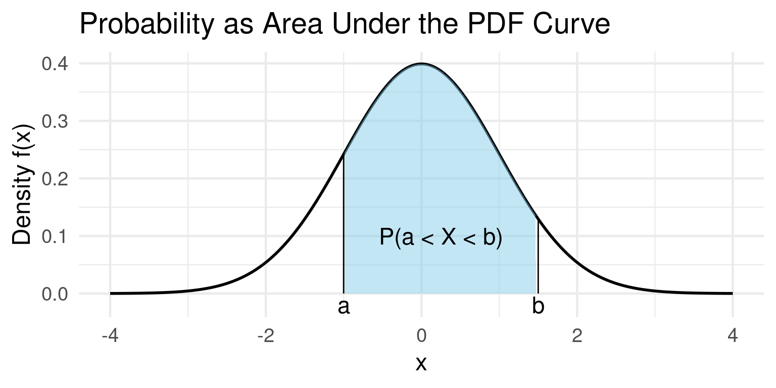
Probability Density Function (PDF)
- For a continuous random variable, the probability of it taking on any single specific value is zero! \(P(X = x) = 0\).
- Why? Because there are infinitely many possible values.
- Instead, we use a Probability Density Function (PDF), \(f(x)\).
- Key Idea: Probability is represented by the area under the curve of the PDF.
Definition: PDF (Informal)
\[ P(a \leq X \leq b) = \text{ Area under $f(x)$ between $a$ and $b$} \]
Example PDF
Example PDF
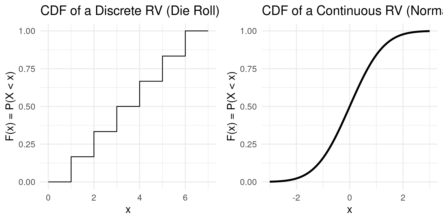
Cumulative Distribution Function (CDF)
- The Cumulative Distribution Function (CDF), \(F(x)\), gives the probability that a random variable \(X\) is less than or equal to a certain value \(x\).
- It’s a unifying concept for both discrete and continuous variables.
Definition: CDF
\[F(x) = P(X \le x)\]
- Properties:
- \(F(x)\) is non-decreasing.
- \(F(x)\) ranges from 0 to 1.
- For continuous RVs, \(P(a \leq X \leq b) = F(b) - F(a)\).
Example CDF
Example: CDF
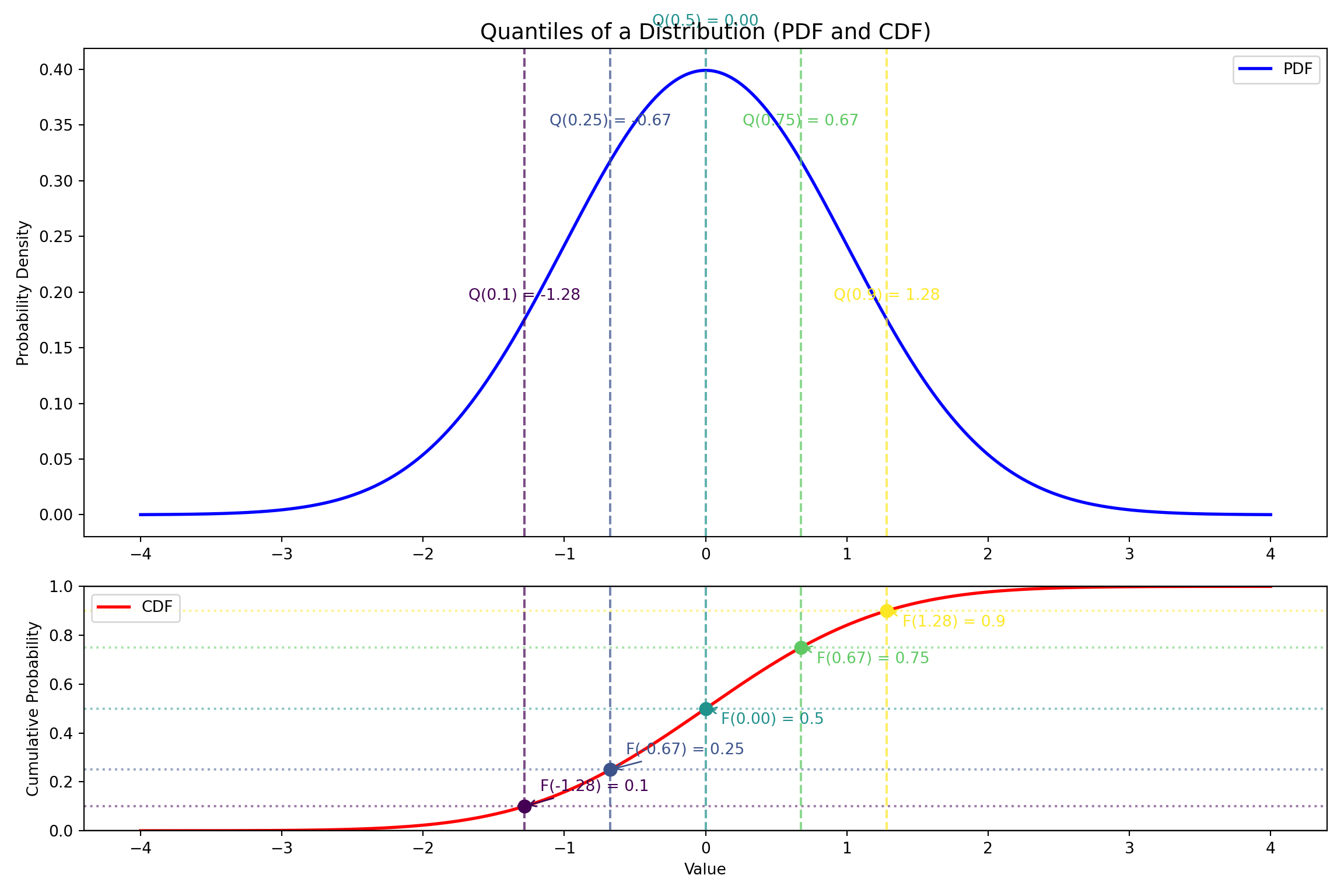
Quantiles of a CDF
Quantiles
- Quantiles are cut points that divide the range of a probability distribution into continuous intervals with equal probabilities.
Definition: Quantile
The \(\tau\)-th quantile (where \(0 < \tau < 1\)) of a random variable \(X\), is the value \(x\) such that the probability of the random variable being less than or equal to \(x\) is \(\tau\).
Mathematically, this is expressed using the Cumulative Distribution Function (CDF), \(F(x)\):
\[ P(X \leq Q(\tau)) = F(Q(\tau)) = \tau \] This means the quantile function, \(Q(\tau)\), is the inverse of the CDF: \(Q(\tau)=F^{-1}(\tau)\)
Quantiles: Visualization
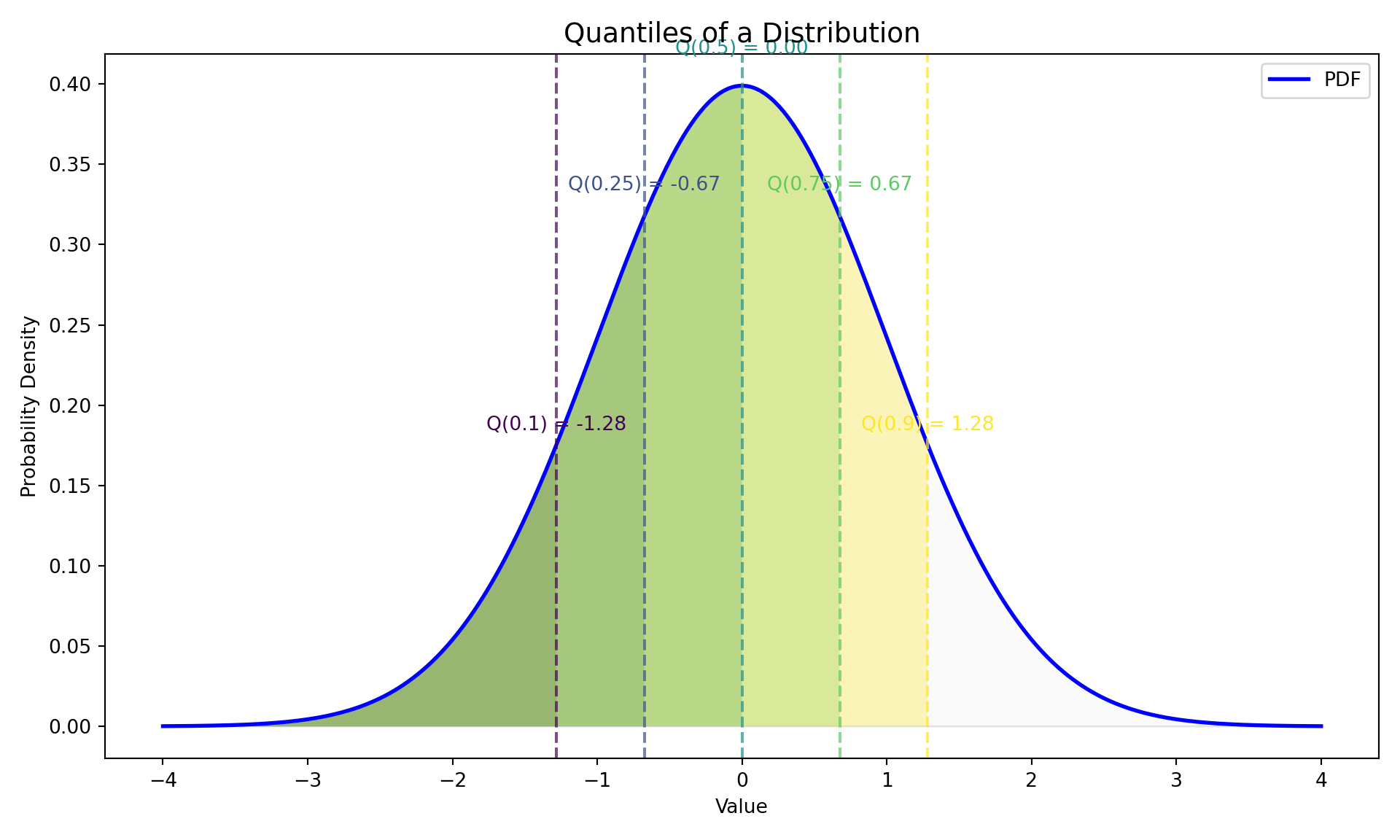
Quantiles via the CDF
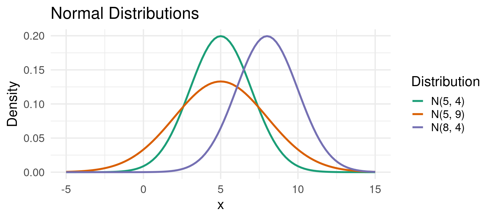
The Normal Distribution
The Normal Distribution
The Normal Distribution is the most important probability distribution in statistics and econometrics.
It is defined by its mean \(\mu\) and its variance \(\sigma^2\).
We write \(X \sim N(\mu, \sigma^2)\).
Properties:
- Bell-shaped and symmetric around its mean \(\mu\).
- Mean = Median = Mode.
- The curve is completely determined by \(\mu\) (center) and \(\sigma\) (spread).
Example Normal Distribution
Example: Normal Distributions
Linear Combinations of Normal Variables
- An important property of the normal distribution is that linear combinations of independent normal variables are also normally distributed.
Theorem: Transformations of Normal Variables
- If \(X \sim N(\mu, \sigma^2)\), then the new variable \(Y = aX + b\) is also normally distributed:
\[Y \sim N(a\mu + b, a^2\sigma^2)\] Note that the new standard deviation is \(|a|\sigma\).
Linear Combinations of Normal Variables
- In the special case of independent normal variables:
Sum/Difference of Independent Variables
If \(X \sim N(\mu_X, \sigma_X^2)\) and \(Y \sim N(\mu_Y, \sigma_Y^2)\) are independent, then their sum and difference are also normally distributed: \[ X + Y \sim N(\mu_X + \mu_Y, \sigma_X^2 + \sigma_Y^2) \] \[ X - Y \sim N(\mu_X - \mu_Y, \sigma_X^2 + \sigma_Y^2) \]
- Key point: Variances always add, even when subtracting the random variables.
Example
Example: Normally Distributed Tasks
Let the time to complete Task A be \(T_A \sim N(20, 3^2)\) minutes and Task B be \(T_B \sim N(15, 4^2)\) minutes. What is the distribution of the total time \(T_{total} = T_A + T_B\)?
- New Mean: \(\mu_{total} = \mu_A + \mu_B = 20 + 15 = 35\)
- New Variance: \(\sigma^2_{total} = \sigma_A^2 + \sigma_B^2 = 3^2 + 4^2 = 9 + 16 = 25\)
- New Standard Deviation: \(\sigma_{total} = \sqrt{25} = 5\)
So, \(T_{total} \sim N(35, 5^2)\). We can now calculate probabilities for the total time, e.g., the probability the total time is less than 45 minutes:
The Standard Normal Distribution (Z)
- The Standard Normal Distribution is a special case of the normal distribution with a mean of 0 and a variance of 1. \(Z \sim N(0, 1)\).
Definition: Standardization
We can convert any normally distributed random variable \(X \sim N(\mu, \sigma^2)\) into a standard normal variable \(Z\) using the formula:
\[ Z = \frac{X - \mu}{\sigma} \]
- It allows us to use a single table (or software function) to find probabilities for any normal distribution.
- The Z-score tells us how many standard deviations an observation \(X\) is away from its mean \(\mu\).
Finding Probabilities
Historically, probabilities for the standard normal distribution were found using Z-tables, which provide \(P(Z \leq z)\).
Today, we use software like R, Stata, or Python.
Finding Normal Probabilities
Example: Suppose annual returns on a mutual fund are normally distributed with a mean of 8% and a standard deviation of 10%. \(X \sim N(0.08, 0.01)\). What’s the probability of a negative return, \(P(X < 0)\)?
Standardize the value: \(Z = (0 - 0.08) / 0.10 = -0.8\)
Find the probability: We need to find \(P(X < 0) = P(\frac{X - 0.08}{0.01} < \frac{0-0.08}{0.01}) = P(Z < -0.8)\).
Finding Probabilities (Cont.)
Finding Normal Probabilities with Software
Using R, Python or Stata: The pnorm() (R) and norm.cdf (Python) functions give the area to the left of the provided value (the CDF).
So, there is about a 21.2% chance of experiencing a negative return.
Conditional Density
Conditional Probability
Conditional probability is about how the probability of an event \(A\) changes when we know an event \(B\) has occurred.
Discrete Case: We update probabilities for specific outcomes. \[ P(A|B) = \frac{P(A \cap B)}{P(B)} \]
Continuous Case: What if we want to condition on a continuous random variable \(Y\) taking a specific value \(y\)?
Since \(P(Y=y) = 0\) for any continuous variable, the formula above is undefined.
We need to shift our thinking from the probability of events to the probability density functions (PDFs) of random variables.
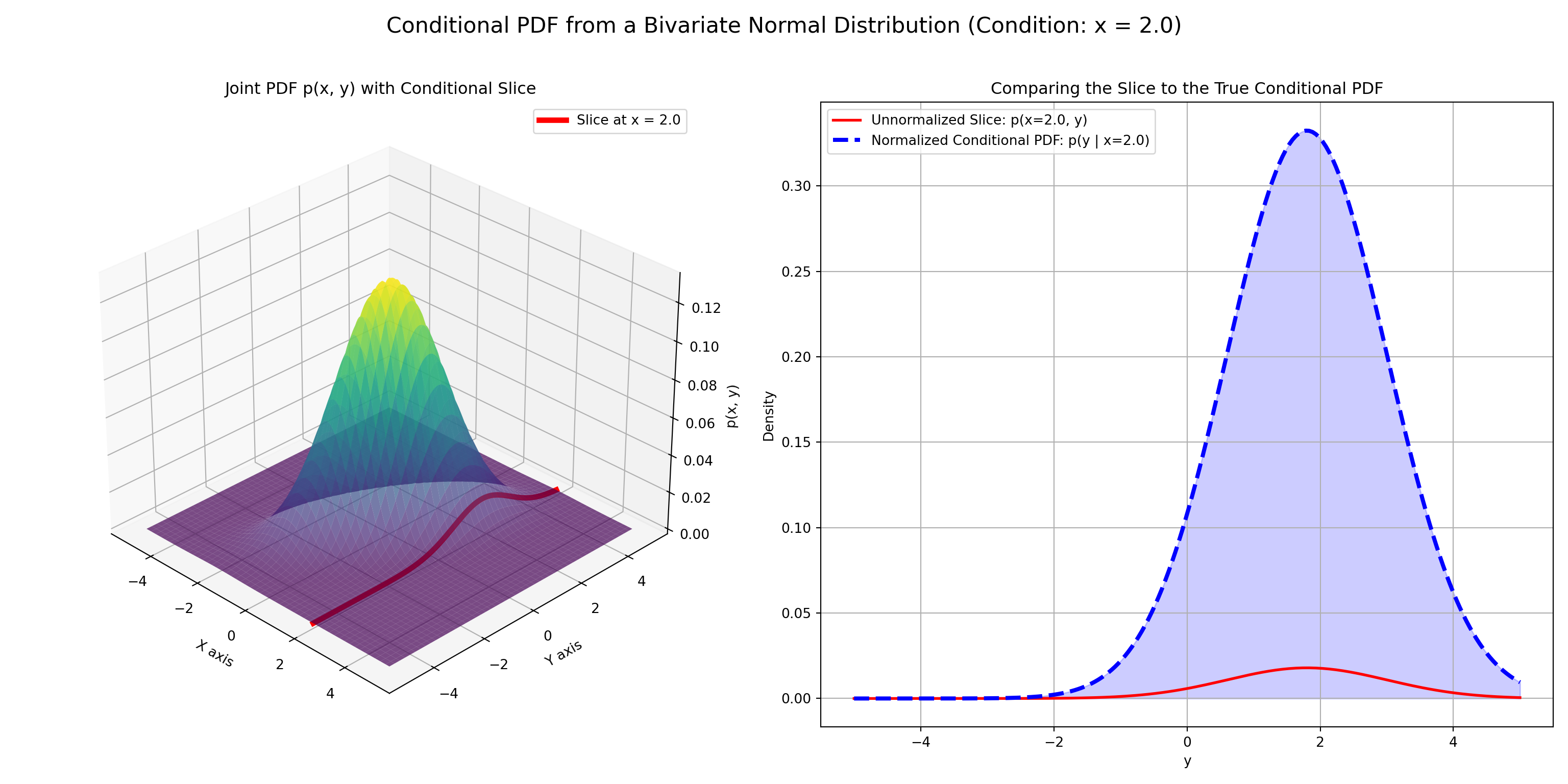
Conditional Probability Density Functions (PDFs)
Definition: Conditional PDF
The conditional PDF of a random variable \(X\) given that \(Y=y\) is defined as the ratio of the joint PDF to the marginal PDF of \(Y\).
\[ f_{X|Y}(x|y) = \frac{f_{X,Y}(x,y)}{f_Y(y)} \]
Provided that the marginal density \(f_Y(y) > 0\).
Similarly, \(f_{X,Y}(x,y)\), the joint PDF, describes the probability density of \((X, Y)\) occurring together.
\(f_Y(y) = \int_{-\infty}^{\infty} f_{X,Y}(x,y) \, dx\): The marginal PDF of \(Y\) found by “integrating out” \(X\). It represents the distribution of \(Y\) on its own.
Intuition: Slicing the Joint Distribution
Think of the joint PDF \(f_{X,Y}(x,y)\) as a 3D surface.
- Fix a value \(y\) for the variable \(Y\). This is like taking a 2D “slice” of the 3D surface at that \(y\).
- The shape of this slice gives the relative likelihood of \(X\)’s values, given that \(Y=y\).
- Normalize the slice: The area under this slice might not be 1. Dividing by \(f_Y(y)\) (the area of the slice) scales it to become a valid probability density function.
This normalized slice is the conditional PDF, \(f_{X|Y}(x|y)\).
Example: Visualization
Visualization of the Conditional PDF
Conditional Expectation
- Conditional expectation, \(E[X | Y=y]\), is simply the expected value (the mean) of
Xcalculated using its conditional distribution.- It’s the “center of mass” of that conditional slice we just discussed.
Definition: Conditional Expectation
Discrete case: if X and Y are discrete random variables, the expectation of X given Y=y is a weighted average using conditional probabilities:
\[ E[X | Y=y] = \sum_{x} x \cdot P(X=x | Y=y) \]
Continuous case: if X and Y are continuous random variables, the expectation is an integral using the conditional PDF:
\[ E[X | Y=y] = \int_{-\infty}^{\infty} x \cdot f_{X|Y}(x|y) \, dx \]
A Crucial Distinction: \(E[X|Y=y]\) vs. \(E[X|Y]\)
\(E[X|Y=y]\) is a function
The expression \(E[X|Y=y]\) produces a value that depends on the specific, fixed
ywe conditioned on. We can think of this as a function of \(y\).
Example \(E[X|Y=y]\)
Let’s define a function \(g(y)\): \[ g(y) = E[X|Y=y] \]
If we know
Y=2, we calculate \(g(2) = E[X|Y=2]\).If we know
Y=5, we calculate \(g(5) = E[X|Y=5]\).
\(E[X|Y]\) is a Random Variable
The notation \(E[X|Y]\) (without specifying a value for \(Y\)) represents a new random variable.
It is the random variable you get by taking the function \(g(y)\) and plugging in the random variable \(Y\) itself. \[ E[X|Y] = g(Y) \]
The value of this new random variable is not known until the value of \(Y\) is revealed.
Example \(E[X|Y]\)
Suppose we find that the expected height of a child \(X\) given the mother’s height \(Y\) is \(E[X|Y=y] = 40 + 0.8y\).
- \(g(y) = 40 + 0.8y\) is the function.
- \(E[X|Y] = 40 + 0.8Y\) is a random variable whose outcome depends on the randomly selected mother’s height \(Y\).
Covariance and Correlation
Covariance
- Covariance measures the joint variability of two random variables. It tells us the direction of the linear relationship.
Definition: Covariance
\[ Cov(X, Y) = \sigma_{XY} = E[(X-\mu_X)(Y-\mu_Y)] \]
- \(Cov(X, Y) > 0\): \(X\) and \(Y\) tend to move in the same direction. When \(X\) is above its mean, \(Y\) tends to be above its mean.
- \(Cov(X, Y) < 0\): \(X\) and \(Y\) tend to move in opposite directions.
- \(Cov(X, Y) = 0\): No linear relationship between \(X\) and \(Y\).
- Drawback: The magnitude of covariance is hard to interpret because it depends on the units of \(X\) and \(Y\). (e.g., Cov(GDP, Consumption) will be a huge number).
Correlation
- The Correlation Coefficient (\(\rho\) or \(r\)) is a standardized version of covariance that measures both the strength and direction of the linear relationship between two variables.
Definition: Correlation
\[ \rho_{XY} = \frac{Cov(X, Y)}{\sigma_X \sigma_Y} \]
- Properties:
- Ranges from -1 to +1.
- \(\rho = +1\): Perfect positive linear relationship.
- \(\rho = -1\): Perfect negative linear relationship.
- \(\rho = 0\): No linear relationship.
- It is unitless, making it easy to interpret and compare.
Example: Correlation
Example: Correlations
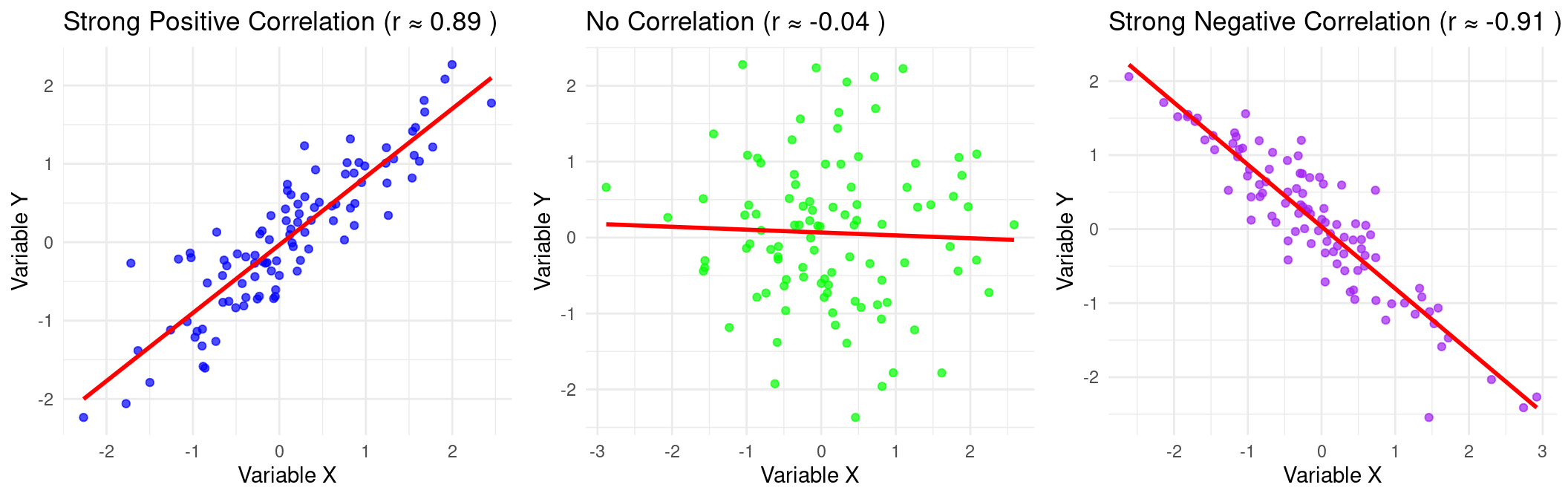
Correlation \(\neq\) Causation
- Reminder: a strong correlation between two variables does not mean that one causes the other. There could be:
- Reverse Causality: \(Y\) causes \(X\).
- Omitted Variable Bias (Lurking Variable): A third variable \(Z\) causes both \(X\) and \(Y\).
Example: Correlation \(\neq\) Causation
- Ice cream sales (\(X\)) and drowning deaths (\(Y\)) are highly positively correlated.
- Does eating ice cream cause drowning? No.
- The omitted variable is hot weather (\(Z\)), which causes people to both buy more ice cream and swim more (leading to more drownings).
Sums of Random Variables
Expected Value
- These rules are fundamental and apply to all random variables, discrete or continuous.
Theorem: Linearity of Expectation
Let \(X\) and \(Y\) be two random variables with means \(\mu_X\) and \(\mu_Y\), and variances \(\sigma_X^2\) and \(\sigma_Y^2\). Let \(a\) and \(b\) be constants.
The expectation of a linear combination is the linear combination of the expectations.
\[ E[aX + bY] = aE[X] + bE[Y] \]
- This rule holds regardless of whether \(X\) and \(Y\) are independent. Expectations are always additive/subtractive in this straightforward way.
Variance
- The rule for variance includes a covariance term.
Theorem: Sum of Variances
The sum of the variances equals:
\[ \text{Var}(aX + bY) = a^2\text{Var}(X) + b^2\text{Var}(Y) + 2ab\,\text{Cov}(X, Y) \]
If \(X\) and \(Y\) are independent random variables, then their covariance is zero (\(\text{Cov}(X, Y) = 0\)). The formula simplifies significantly:
\[ \text{Var}(aX + bY) = a^2\text{Var}(X) + b^2\text{Var}(Y) \]
Simple Cases (for Independent Variables):
- Sum: \(\text{Var}(X + Y) = \text{Var}(X) + \text{Var}(Y)\)
- Difference: \(\text{Var}(X - Y) = \text{Var}(X) + \text{Var}(Y)\)
Covariance
- Covariance of sums can also be decomposed as sums of covariances.
Sums of Covariances
The covariance can be decomposed as: \[ \text{Cov}(aX + bY, Z) = a\,\text{Cov}(X, Z) + b\,\text{Cov}(Y, Z) \]
In addition, the covariance of \(X\) with itself equals the variance:
\[ \text{Cov}(X, X) = \text{Var}(X) \]
Covariance Example
Example: Proof that \(\text{Var}(X+Y)=\text{Cov}(X+Y, X+Y)\)
We know that \(\text{Var}(X+Y) = \text{Var}(X) + \text{Var}(Y) + 2 \text{Cov}(X,Y)\) by definition.
Now observe that:
\[\begin{align*} \text{Cov}(X+Y, X+Y) &= \text{Cov}(X,X+Y)+\text{Cov}(Y,X+Y) \newline &= \text{Var}(X)+\text{Cov}(X,Y)+\text{Cov}(Y,X)+\text{Var}(Y) \newline &= \text{Var}(X)+\text{Var}(Y)+2\text{Cov}(X,Y) \end{align*}\]
..which is equal to \(\text{Var}(X+Y)\).
Summary Table
The following table outlines the results previously discussed:
| Property | Linear Combination | General Case | Independent Case (\(Cov(X,Y)=0\)) |
|---|---|---|---|
| Expectation | \(E[aX \pm bY]\) | \(a\mu_X \pm b\mu_Y\) | (Same as General) |
| \(E[X + Y]\) | \(\mu_X + \mu_Y\) | (Same as General) | |
| \(E[X - Y]\) | \(\mu_X - \mu_Y\) | (Same as General) | |
| Variance | \(\text{Var}(aX + bY)\) | \(a^2\sigma_X^2 + b^2\sigma_Y^2 + 2ab\,\text{Cov}(X,Y)\) | \(a^2\sigma_X^2 + b^2\sigma_Y^2\) |
| \(\text{Var}(X + Y)\) | \(\sigma_X^2 + \sigma_Y^2 + 2\,\text{Cov}(X,Y)\) | \(\sigma_X^2 + \sigma_Y^2\) | |
| \(\text{Var}(X - Y)\) | \(\sigma_X^2 + \sigma_Y^2 - 2\,\text{Cov}(X,Y)\) | \(\sigma_X^2 + \sigma_Y^2\) |
Summary
What did we do?
- Probability Concepts:
- The lecture began by introducing foundational probability concepts, including experiments, sample spaces, events, and the rules for calculating probabilities of unions, intersections, and conditional events (\(P(A|B)\)).
- Dicsrete and Continuous Distributions:
- We defined discrete and continuous random variables and their key descriptive functions: the Probability Mass/Density Function (PMF/PDF) and the Cumulative Distribution Function (CDF). This section also covered how to calculate the expected value (\(E[X]\)) and variance (\(Var(X)\)) of a random variable.
- The Normal Distribution:
- A significant portion was dedicated to the Normal distribution, explaining its properties, the importance of its parameters (mean and variance), and how any normal variable can be standardized into a Z-score. It also covered the properties of linear combinations of normal variables.
What did we do? (Cont.)
- Conditional Distributions:
- The relationship between variables was explored through multiple lenses, including conditional probability density functions (\(f_{X|Y}(x|y)\)), conditional expectation (\(E[X|Y]\)), and measures of linear association like covariance and correlation, while reiterating the crucial distinction that correlation does not imply causation.
- Rules for Expected Value and Variance:
- Finally, the lecture established the mathematical rules for the expectation and variance of sums of random variables. It detailed the linearity of expectation and the formula for the variance of a sum, emphasizing the simplification that occurs when the variables are independent and their covariance is zero.
Inferential Statistics
Population vs. Sample
- In the previous lecture, we have seen concepts like expected values, \(E[X]\) or \(\mu_X\), and variances \(\sigma^2\).
- These are parameters that belong to a population: the entire group of individuals, objects, or data points that we are interested in studying.
- In reality, we usually only have a sample, a subset of the population from which we actually collect data, at our disposal.
- It’s often impossible or too expensive to collect data on the entire population. We use samples to make inferences about the population.
Example Populations and Samples
- Populations:
- All households in the United States.
- All firms listed on the New York Stock Exchange.
- Samples:
- A survey of 2,000 U.S. households.
- The stock prices of 50 firms from the NYSE.
Parameters vs. Statistics
- The core idea of inference is to use a sample statistic to learn about a population parameter.
Definition: Parameter
A parameter is a numerical characteristic of a population. These are typically unknown and what we want to estimate. They are considered fixed values.
Example: Parameters
The population mean (\(\mu\)), population variance (\(\sigma^2\)), population correlation (\(\rho\)).
Statistics
- The core idea of inference is to use a sample statistic to learn about a population parameter.
Definition: Statistic
A numerical characteristic of a sample. We calculate statistics from our data. A statistic is a random variable, as its value depends on the particular sample drawn.
Example: Statistics
Sample mean (\(\bar{x}\)), sample variance (\(s^2\)), sample correlation (\(r\)).
The Concept of a Sampling Distribution
Simple Random Sampling
In statistics, we usually want to compute a statistic and derive its distribution to say something about a corresponding parameter in the population. To do so, we need to assume things about the way our data is sampled.
Simple Random Sampling (SRS) is the most basic sampling method.
Defintion: Simple Random Sampling
A sample of size \(n\) where every possible sample of that size has an equal chance of being selected, and every individual in the population has an equal chance of being included.
- SRS is the ideal. Statistical methods (like the ones we’re learning) are built on the assumption of random sampling.
- If a sample is not drawn randomly, our inferences may be biased and incorrect.
The Distribution of a Statistic
- This is a crucial, but sometimes tricky, concept.
Thought Experiment
- There is a population with an unknown mean \(\mu\).
- We take a random sample of size \(n\) (e.g., n=100) and calculate its sample mean, \(\bar{x}_1\).
- We take a different random sample of size \(n\) and get a different sample mean, \(\bar{x}_2\).
- We repeat this process 10,000 times, getting \(\bar{x}_1\), \(\bar{x}_2\), \(\dots\), \(\bar{x}_{10000}\).
- The Sampling Distribution of the a statistic (in this case the sample mean) is the probability distribution of all these possible \(\bar{x}\) values. It’s the distribution of a statistic, not of the original data.
Sampling Distribution Simulation
Code
set.seed(42)
population_mean <- 50
population_sd <- 10
sample_size <- 100
num_samples <- 10000

sample_means <- replicate(num_samples, mean(rnorm(sample_size, mean = population_mean, sd = population_sd)))

hist(sample_means,
     breaks = 50,
     main = "Distribution of Sample Means",
     xlab = "Sample Mean",
     ylab = "Frequency",
     col = "lightblue",
     border = "black")
abline(v = population_mean, col = "red", lty = 2, lwd = 2)
grid()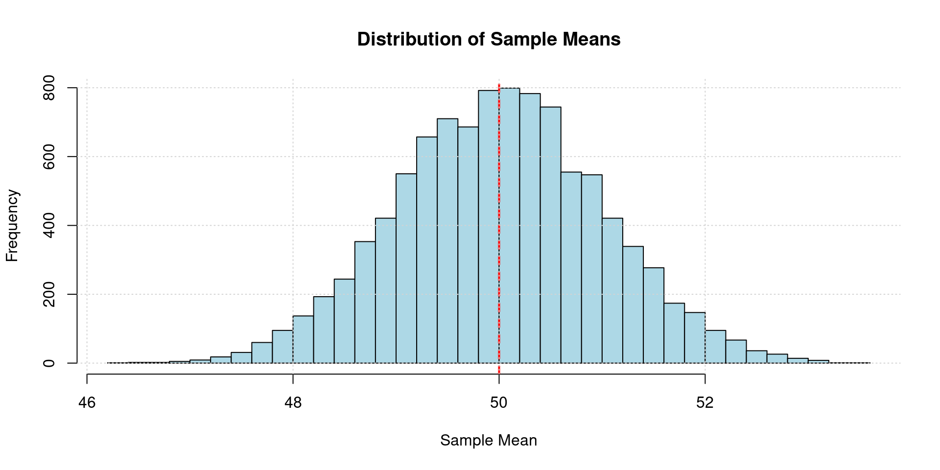
Code
import numpy as np
import matplotlib.pyplot as plt

np.random.seed(42)
population_mean, population_std, sample_size, num_samples = 50, 10, 100, 10000
sample_means = [np.mean(np.random.normal(loc=population_mean, scale=population_std, size=sample_size)) for _ in range(num_samples)]

plt.figure(figsize=(10, 6))
plt.hist(sample_means, bins=50, edgecolor='black', alpha=0.7)
plt.axvline(x=population_mean, color='red', linestyle='--', linewidth=2)
plt.title('Distribution of Sample Means')
plt.xlabel('Sample Mean')
plt.ylabel('Frequency')
plt.grid(True, alpha=0.3)
plt.show()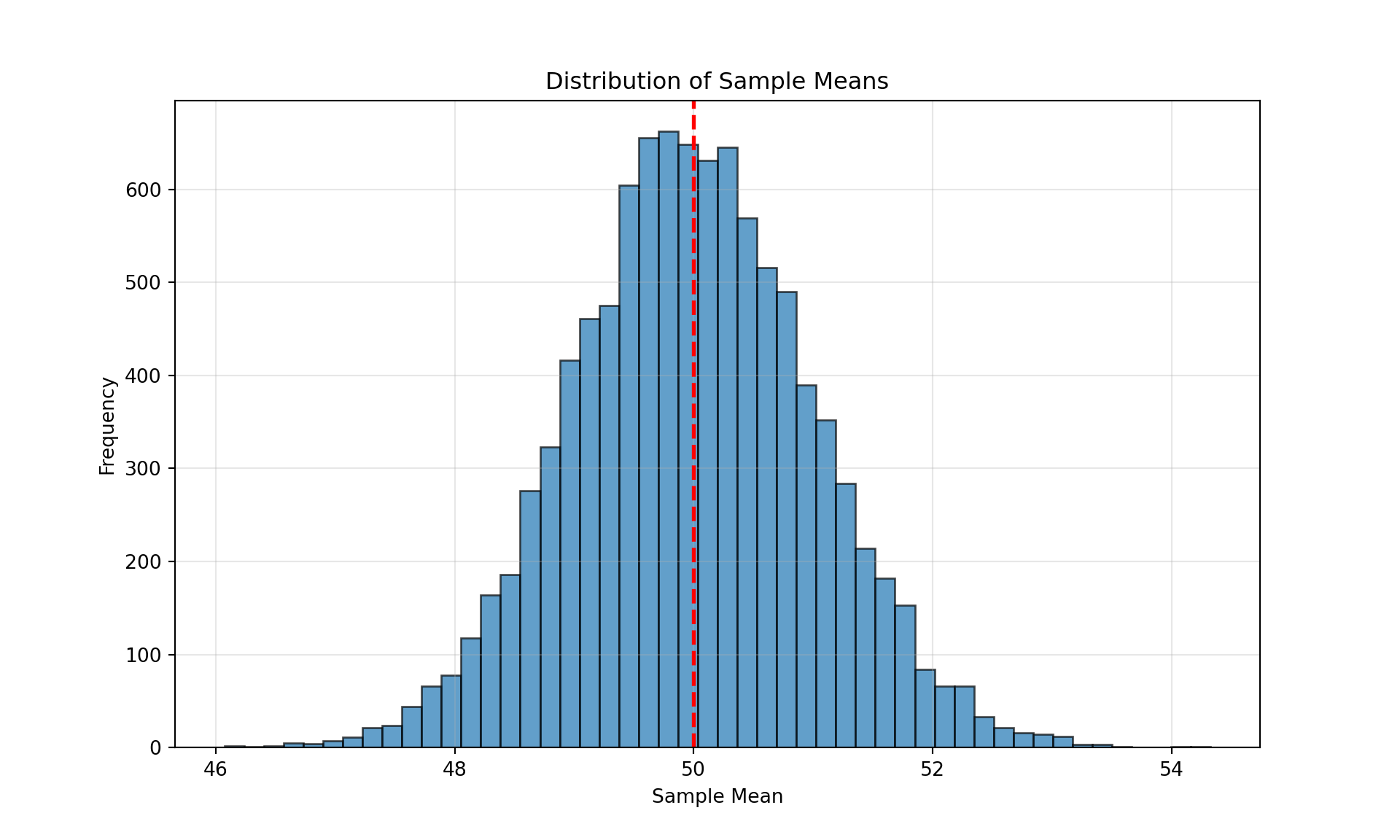
Code
clear all
set seed 42
set obs 10000
* Parameters
scalar population_mean = 50
scalar population_sd = 10
scalar sample_size = 100
* Generate sample means
gen sample_mean = .
quietly {
forvalues i = 1/10000 {
drawnorm x, n(`=sample_size') mean(`=population_mean') sd(`=population_sd') clear
summarize x
replace sample_mean = r(mean) in `i'
}
}
* Plot histogram
histogram sample_mean, ///
bin(50) ///
title("Distribution of Sample Means") ///
xtitle("Sample Mean") ///
ytitle("Frequency") ///
fcolor("lightblue") ///
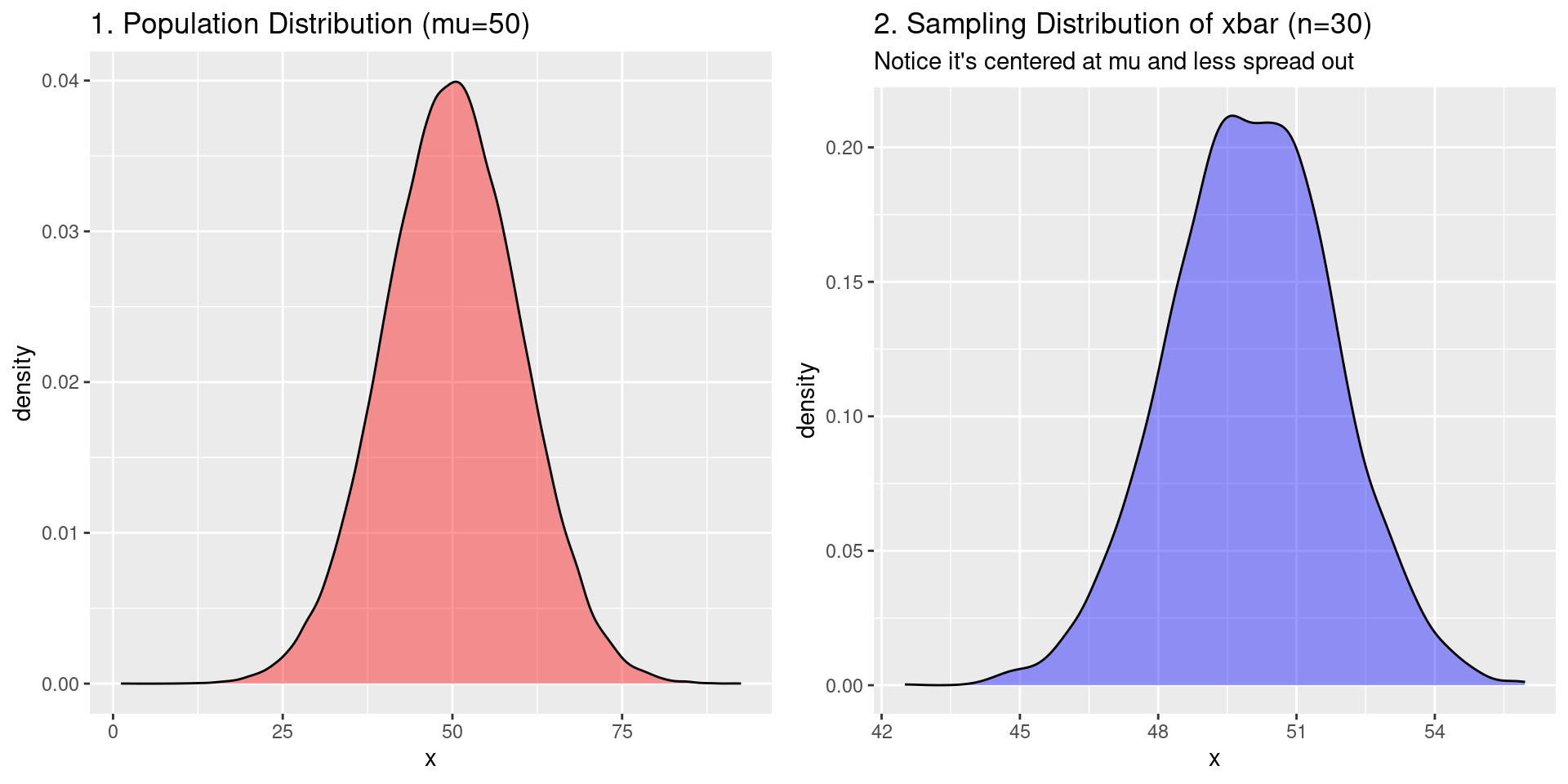
addplot(pci 0 0 `=population_mean' `=population_mean', lcolor(red) lpattern(dash))Sampling Distribution Visualization
- On the left: the distribution of \(X\) in the population
- On the right: the distribution of \(\bar{X}\)
Sampling Distribution Example
Numerical Example Sampling Distribution
Imagine a tiny population that contains only four numbers. These are all the values that exist in our entire population.
[1] "The population is: 2, 4, 6, 10"[1] "The true population mean (mu) is: 5.5"The true mean of our population is 5.5. In a real research problem, this is the value we want to estimate, but we don’t know it.
Now, let’s list every single possible sample of size \(n = 2\) that we can draw from this population without replacement.
The number of combinations is “4 choose 2”, which is 6. We can use R to list them all.
[1] "All 6 possible samples of size n=2:" [,1] [,2] [,3] [,4] [,5] [,6]
[1,] 2 2 2 4 4 6
[2,] 4 6 10 6 10 10Sampling Distribution Example (Cont.)
Numerical Example Sampling Distribution (Cont.)
For each of the 6 possible samples, we will now calculate its sample mean (\(\bar{x}\)).
[1] "The mean of each of the 6 possible samples:"[1] 3 4 6 5 7 8The list of all possible sample means we just calculated (3, 4, 6, 5, 7, 8) is the sampling distribution of the sample mean. This gives the distribution of all possible values the sample mean can take for a sample of size \(n=2\) from our population. Since we assume SRS, each outcome is equally likely.
Let’s organize it into a frequency table and visualize it.
[1] "The Sampling Distribution (as a frequency table):" Sample_Mean Frequency
1 3 1
2 4 1
3 5 1
4 6 1
5 7 1
6 8 1Visualization the Sampling Distribution
- We can again visualize this distribution with a histogram.
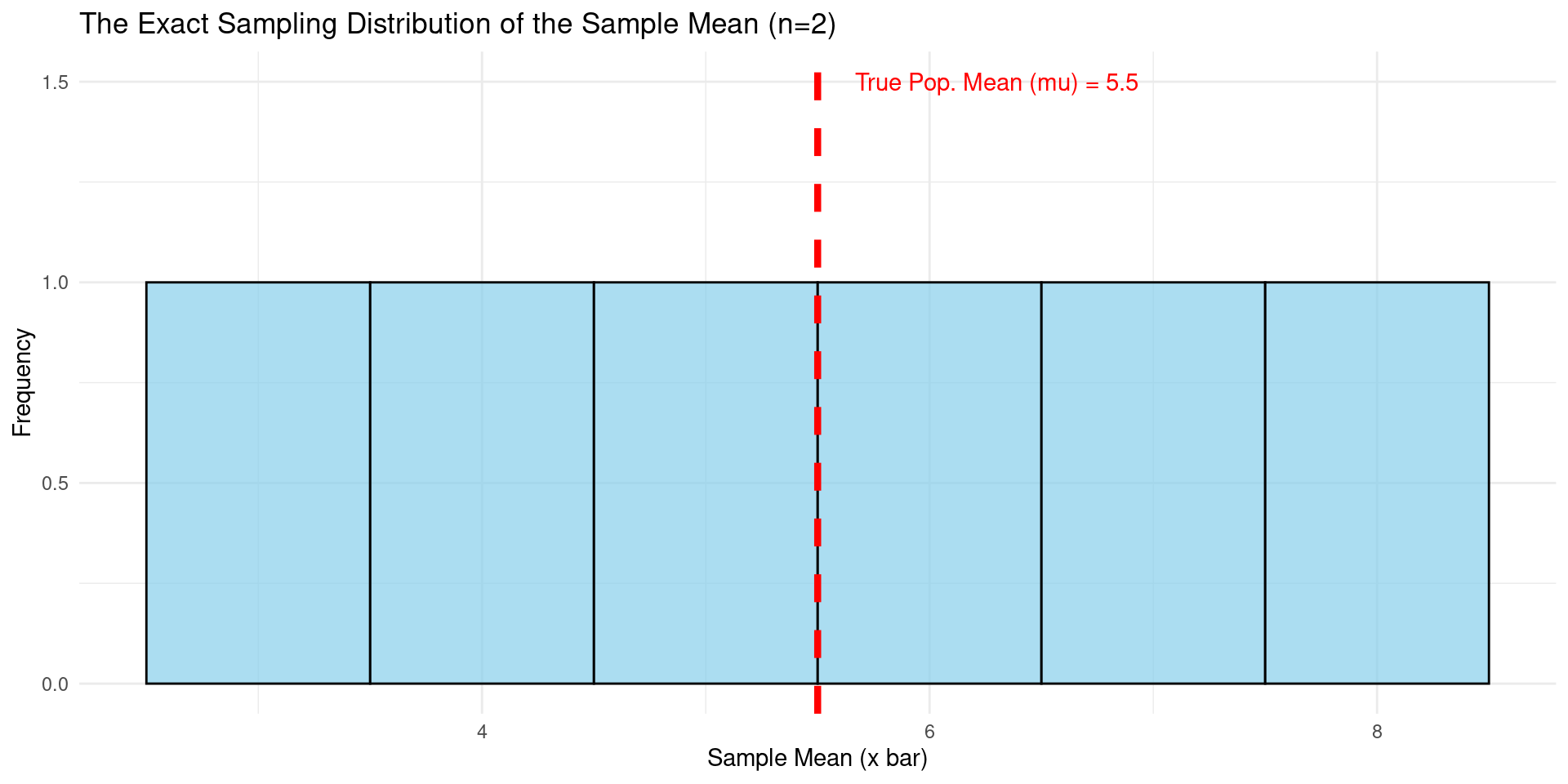
- The explicit PMF of the sampling distribution is the normalized version of this histogram: \(P(\bar{X}=3)=\frac{1}{6}, P(\bar{X}=4)=\frac{1}{6}, \dots, P(\bar{X}=8)=\frac{1}{6}\).
The Central Limit Theorem (CLT)
The Central Limit Theorem
- The Central Limit Theorem (CLT) states:
Theorem: Central Limit Theorem
If you take a sufficiently large random sample (\(n \geq 30\) is a common rule of thumb) from a population distributed with mean \(\mu\) and standard deviation \(\sigma\), the sampling distribution of the sample mean \(\bar{x}\) will be approximately normally distributed, regardless of the original population’s distribution.
Furthermore, the mean of this sampling distribution will be the population mean \(\mu\), and its standard deviation (called the standard error) will be \(\sigma / \sqrt n\).
\[\bar{X} \approx N\left(\mu, \frac{\sigma^2}{n}\right)\]
Why Is The CLT Important?
The implications of the CLT are profound:
We can use the normal distribution for inference on the mean even if the underlying data is not normal. Many economic variables (like income) are highly skewed, but the CLT lets us work with their sample means.
It provides a precise formula for the variance of the sample mean (\(\sigma^2/n\)). This shows that as our sample size \(n\) increases, the sample mean \(\bar{x}\) becomes a more precise estimator of the population mean \(\mu\) (its sampling distribution gets narrower).
The CLT is the foundation that allows us to build confidence intervals and conduct hypothesis tests for the mean. And later, also for estimators that are functions of the mean.
Example of the CLT
Example: Poisson-distributed RV’s
Let \(X_1, \dots, X_n\) be independent, identically distributed (i.i.d.) random variables following a Poisson distribution with parameter \(\lambda\), i.e., \(X_i \sim \text{Poisson}(\lambda)\). The Poisson distribution has mean \(E[X_i]=\lambda\) and Variance \(\text{Var}(X_i)=\lambda\).
By the CLT, \(\frac{1}{n} \sum_{i=1}^n X_i = \bar{X}_n \sim N(\lambda, \frac{\lambda}{n})\).
Suppose that \(\lambda=5\) and \(N=100\), then \(\bar{X}_n \sim N(5,\frac{5}{100})=N(5,0.05).\) In the simulation below, where we plot 10000 simulations of \(\bar{X}_n\), we should find that the empirical mean is 5 and the empirical variance is 0.05.
Code
set.seed(123)  # For reproducibility
lambda <- 5    # Poisson parameter
n <- 100       # Sample size
n_sim <- 10000 # Number of simulations

# Simulate 10,000 sample means (each from n=100 Poisson(5) samples)
x_bars <- replicate(n_sim, mean(rpois(n, lambda)))

# Compute empirical mean and variance of x_bars
empirical_mean <- mean(x_bars)
empirical_var <- var(x_bars)

cat("Empirical Mean:", empirical_mean, "Empirical Var:", empirical_var)
Empirical Mean: 4.996629 Empirical Var: 0.04879321Code
import numpy as np
import matplotlib.pyplot as plt
from scipy.stats import norm

# Set random seed for reproducibility
np.random.seed(123)

# Parameters
lambda_ = 5     # Poisson parameter
n = 100         # Sample size
n_sim = 10000   # Number of simulations

# Simulate 10,000 sample means (each from n=100 Poisson(5) samples)
x_bars = np.array([np.random.poisson(lambda_, n).mean() for _ in range(n_sim)])

# Empirical mean and variance
empirical_mean = np.mean(x_bars)
empirical_var = np.var(x_bars, ddof=1)  # ddof=1 for unbiased estimator

# Print results
print(f"Empirical Mean: {empirical_mean:.6f}, Empirical Var: {empirical_var:.6f}")
Empirical Mean: 5.000215, Empirical Var: 0.048941Code
clear
set seed 123
set obs 10000

local lambda = 5
local n = 100
local n_sim = 10000

// Generate 10,000 sample means
gen x_bar = .
forvalues i = 1/`n_sim' {
    qui drawnorm x, n(`n') means(`lambda') sds(sqrt(`lambda')) clear
    qui replace x_bar = r(mean) in `i'
}

// Calculate empirical mean and variance
sum x_bar
di "Empirical Mean: " r(mean) ", Empirical Var: " r(Var)
Estimation and Inference
Point Estimators
Definitions: Estimator, Estimate, Point Estimate
An estimator is a rule (a formula) for calculating an estimate of a population parameter based on sample data. The value it produces is called an estimate.
A point Estimator is a formula that produces a single value/number as the estimate.
- Common Point Estimators:
- The sample mean \(\bar{x}\) is a point estimator for the population mean \(\mu\).
- The sample proportion \(\hat{p}\) is a point estimator for the population proportion \(p\).
- The sample variance \(s^2\) is a point estimator for the population variance \(\sigma^2\).
Desirable Properties of Estimators
- How do we know if an estimator is “good”? We look for three properties (conceptually):
Definition: Unbiasedness
An estimator is unbiased if its expected value is equal to the true population parameter. \(E[\theta]=\theta\).
Analogy: On average, the shots hit the center of the target. There’s no systematic over- or under-estimation.
Definition: Consistency
An estimator is consistent if, as the sample size \(n\) approaches infinity, the value of the estimator converges to the true parameter value.
Analogy: The more information you get, the closer you get to the truth.
Desirable Properties of Estimators (Cont.)
- How do we know if an estimator is “good”? We look for three properties (conceptually):
Definition: Efficiency
Among all unbiased estimators, the most efficient one is the one with the smallest variance.
Analogy: The shots are tightly clustered around the center. It’s a precise estimator.
Hypothesis Testing
- Hypothesis Testing is a formal procedure for checking whether our sample data provides convincing evidence against a preconceived claim about the population.
The Logic: Proof by Contradiction
- We start by assuming something is true about the population (the Null Hypothesis).
- We then look at our sample data.
- We ask: “If the null hypothesis were true, how likely is it that we would get sample data like this?”
- If our sample data is very unlikely under the null hypothesis, we reject our initial assumption in favor of an alternative.
Null and Alternative Hypotheses
Every hypothesis test has two competing hypotheses:
Null Hypothesis (\(H_0\)): The claim being tested. It’s the “status quo” or “no effect” hypothesis. It always contains an equality sign (\(=\), \(\leq\), or \(\geq\)).
Examples: Null Hypothesis \(H_0\)
The new drug has no effect on blood pressure (\(\mu_{change} = 0\)).
The mean income in a region is \(50,000\) (\(\mu = 50000\)).
Alternative Hypothesis
- Alternative Hypothesis (\(H_A\) or \(H_1\)): The claim we are trying to find evidence for. It’s what we conclude if we reject the null hypothesis. It never contains an equality sign (\(\neq\), \(<\), or \(>\)).
Examples: Null Hypothesis \(H_A\)
The new drug does have an effect (\(\mu_{change} \neq 0\)).
The mean income is not \(50,000\) (\(\mu \neq 50000\)).
Test Statistics and \(p\)-values (Conceptual)
How do we decide whether our data is “unlikely”?
Test Statistic: A value calculated from sample data that measures how far our sample statistic (e.g., \(\bar{x}\)) is from the parameter value claimed by the null hypothesis (\(\mu_0\)). It’s often standardized, like a Z-score.
Definition: Test Statistic (Informal)
\[ \text{Test Statistic} = \frac{\text{Sample Statistic} - \text{Null Hypothesis Value}}{\text{Standard Error}} \]
\(p\)-values
Definition: \(p\)-value
The \(p\)-value is the probability of observing a test statistic as extreme (or more extreme) than the one calculated, assuming the null hypothesis is true.
- Small P-Value (e.g., < 0.05): The observed data is very unlikely if \(H_0\) were true. We reject \(H_0\). The evidence supports \(H_A\).
- Large P-Value (e.g., > 0.05): The observed data is plausible if \(H_0\) were true. We fail to reject \(H_0\). There is not enough evidence to support \(H_A\).
A Crucial Ingredient: The Standard Error
- How do we measure if a sample result is “surprising”? We use the Standard Error (SE).
Definition: Standard Error
The Standard Error of a statistic (like the sample mean) is the standard deviation of its sampling distribution. In simpler terms, it measures the typical or average distance between the sample statistic and the true population parameter.
- The SE tells us how much we expect e.g. a sample mean (\(\bar{x}\)) to naturally vary from the true population mean (\(\mu\)).
- A small SE means our sample means will be tightly clustered around the true mean.
- A large SE means they will be more spread out.
One-Sided vs. Two-Sided Hypotheses
Two-Sided Hypotheses tests are the most common type of test.
Is the population parameter different from a specific value? (We don’t care if it’s higher or lower, just that it’s not the same).
- Null Hypothesis: \(H_0: \mu = \mu_0\)
- Alternative Hypothesis: \(H_A: \mu \neq \mu_0\)
- We are looking for an extreme result in either direction.
The significance level (\(\alpha\), e.g., 0.05) is split between the two tails of the distribution.
Definition: Significance level
The significance level, denoted as \(\alpha\), is the probability we are willing to incur of rejecting the null hypothesis when it is actually true.
Rejection Region Two-Sided Test
- We are looking for an extreme result in either direction.
- The significance level (\(\alpha\), e.g., 0.05) is split between the two tails of the distribution.

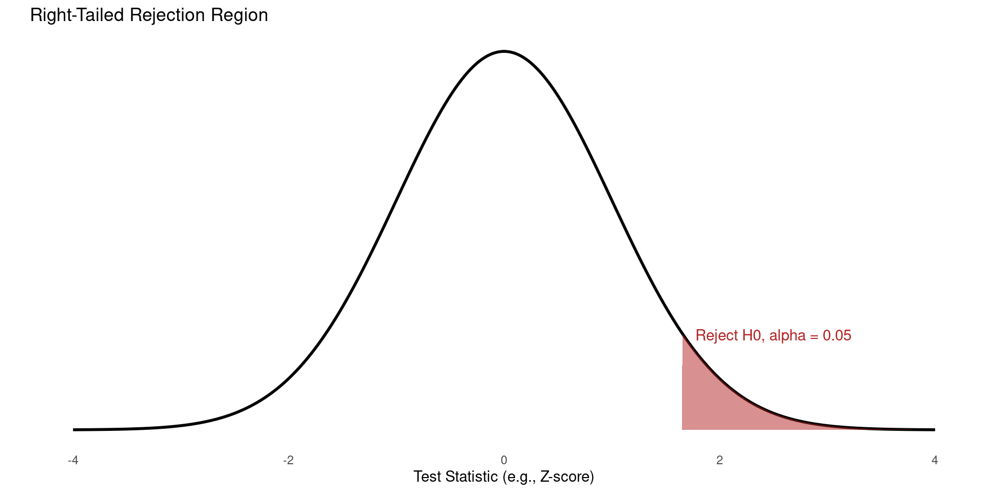
One-Sided Hypothesis Testing (Right-Tailed)
The Question: Is the population parameter greater than a specific value?
This is used when we have a strong reason to believe the effect can only go in one direction, or we are only interested in an effect in one direction.
- Null Hypothesis: \(H_0: \mu \le \mu_0\)
- Alternative Hypothesis: \(H_A: \mu > \mu_0\)
Rejection Region One-Sided Test (Right-Tailed)
- The entire significance level (\(\alpha\)) is placed in the upper (right) tail.
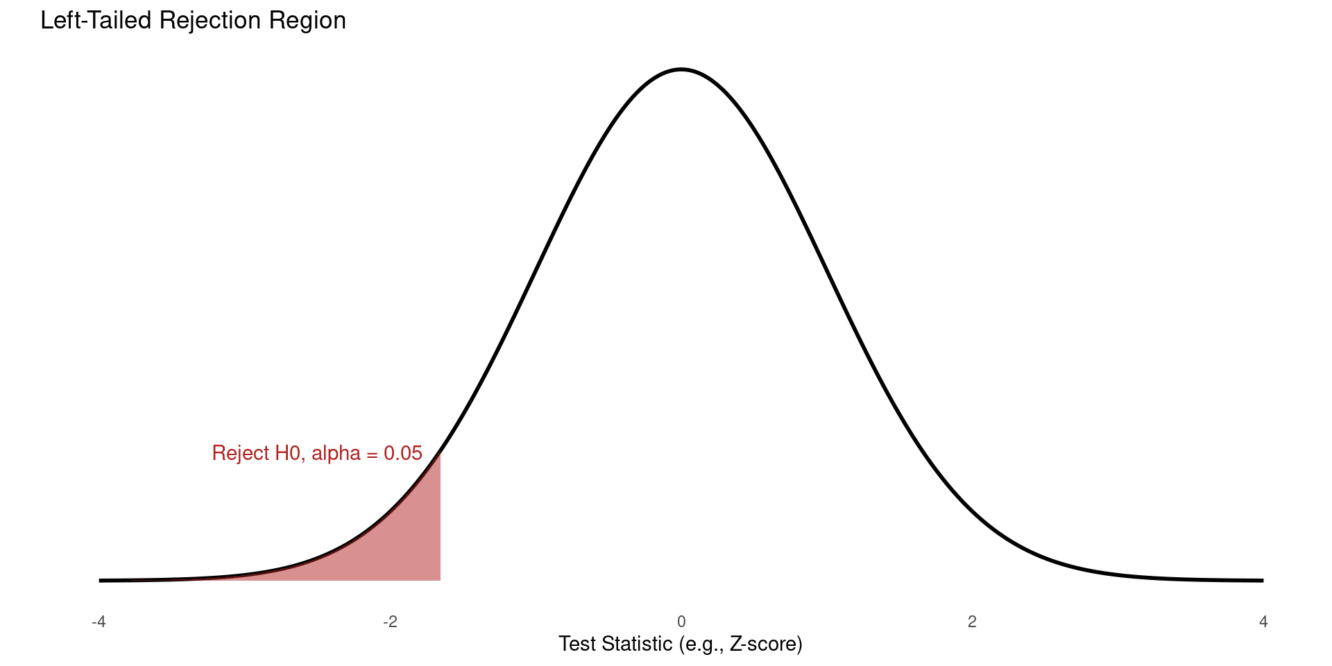
One-Sided Hypothesis Testing (Left-Tailed)
- In the left-tailed case, we ask whether the population parameter is less than a specific value?
- Null Hypothesis: \(H_0: \mu \ge \mu_0\)
- Alternative Hypothesis: \(H_A: \mu < \mu_0\)
Rejection Region One-Sided Test (Left-Tailed)
- The entire significance level (\(\alpha\)) is placed in the lower (left) tail.
Example Hypothesis Testing
Example: Fertilizer
We are testing if a new fertilizer increases or decreases crop yield. We have a dataset of land units that either use fertilizer or not, and their associated crop yields. We have a sample size \(\geq\) 30 in both groups, meaning we can assume the CLT holds.
A good estimator of the crop yield in either group (fertilizer, \(\mu_F\) and no fertilzer \(\mu_N\)) is the group’s sample mean, \(\overline{\mu_F}\) and \(\overline{\mu_N}\). Suppose we also know that both crop yields are distributed around their population means with variance \(\sigma^2=5\).
According to the CLT, we know that \(\overline{\mu_F} \sim N(\mu_F, \frac{5}{30})\) and \(\overline{\mu_N} \sim N(\mu_N, \frac{5}{30})\).
Suppose we want to know whether the group yields differ per group. This is a two-sided hypothesis: \(H_0: \mu_F = \mu_N\), and \(H_A: \mu_F \neq \mu_N\).
Example Hypothesis Testing (Cont.)
Example: Fertilizer (Cont.)
Suppose our test statistic is \(T = \overline{\mu_F} - \overline{\mu_N}\). Under the null hypothesis, its expected value is 0. According to the law of variances, its variance is \(\frac{5}{30} + \frac{5}{30} = \frac{1}{3}\). Since both components are normally distributed, under the null hypothesis our test statistic \(T \sim N(0, \frac{1}{3})\).
Suppose our data show that \(\overline{\mu_F}=5\) and \(\overline{\mu_N}=1\). Hence \(T=4\). How likely is that under the null hypothesis?
\[\begin{align*} P(|T|> 4) &= P(T>4) + P(T<-4) \newline &= P(Z > \frac{4}{\sqrt{\frac{1}{3}}}) + P(Z < \frac{-4}{\sqrt{\frac{1}{3}}}) &\approx 0 \end{align*}\]
This probability is also the \(p\)-value. This means that it is very unlikely to observe this difference between the two groups given the null hypothesis. Therefore, with e.g. \(\alpha=0.05\), we reject the null hypothesis.
Example Hypothesis Testing (Cont.)
Example: Fertilizer (Cont.)
Suppose now that \(\overline{\mu_F}=1.5\) and \(\overline{\mu_N}=1\), such that \(T=0.5\), and we’re interested in whether fertilizer increases crop yield. This is a one-sided hypothesis test with \(H_0: \mu_F = \mu_N\) against \(H_A: \mu_F > \mu_N\). We again use a significance level \(\alpha=0.05\).
Under the null hypothesis, \(T \sim N(0, \frac{1}{3})\). We now calculate the \(p\)-value as \(P(T > 0.5)\) = \(P(Z > \frac{0.5}{\sqrt{\frac{1}{3}}}) = P(Z > 0.86)\), which evaluates to 0.19. Since we have a significance-level of 5%, we do not reject the null hypothesis: the test statistic we observed is not unlikely enough to reject it.
Which Test to Use?
- Golden Rule: Unless you have a very strong, justifiable, pre-specified reason for expecting an effect in only one direction, you should use a two-sided test.
- Two-sided tests define the \(p\)-value as the probability of observing something more extreme than the observed test statistic on both sides, i.e. \(P(|T|>t)\)
- One-sided tests define the \(p\)-value as the probability of observing something more extreme than the observed test statistic on one side, i.e. \(P(T>t)\) or \(P(T<t)\).
| Feature | Two-Sided Test | One-Sided Test |
|---|---|---|
| Key Question | Is there a difference? | Is it greater than or less than? |
| Alternative (\(H_A\)) | \(\mu \neq \mu_0\) | \(\mu > \mu_0\) or \(\mu < \mu_0\) |
| Rejection Region | Split into two tails | All in one tail (left or right) |
| When to Use | The default, conservative choice. | Only when there is a strong prior reason or you only care about one direction. |
| Power | Less powerful. | More powerful (if the effect is in the hypothesized direction). |
Confidence Intervals
Confidence Intervals
Definition: Confidence Interval
A confidence interval (CI) is a range of values, derived from sample data, that is likely to contain the value of an unknown population parameter (e.g., the true population mean \(\mu\) or proportion \(p\)).
- Ingredients:
- Point Estimate: A single value calculated from the sample that estimates the population parameter (e.g., sample mean \(\bar{x}\)). It’s our “best guess,” but it’s almost certainly wrong.
- Interval Estimate: The confidence interval provides a range around the point estimate, acknowledging the uncertainty inherent in sampling.
- Confidence Level: The probability that the method used to construct the interval will capture the true population parameter. Common levels are 90%, 95%, and 99%.
Interpretation
The confidence level refers to the long-run success rate of the method, not the probability of a single interval being correct.
Correct Interpretation: “We are 95% confident that the method used to construct this interval from our sample captures the true population mean.”
- Analogy: Imagine throwing rings at a post (the true parameter). The 95% confidence level means that if you were to take many samples and throw many “ring” intervals, 95% of them would land on the post. You don’t know if the one ring you just threw is a success or a miss.
Incorrect Interpretation: It is wrong to say, “There is a 95% probability that the true population mean lies within this specific interval \([A, B]\).” Once an interval is calculated, the true mean is either in it or it isn’t; there is no probability involved for that specific interval.
Construction of a Confidence Interval
- Most confidence intervals share a common structure.
Construction of a Confidence Interval
\[ CI= \text{Point Estimate} \pm \text{Margin of Error} \]
- The Margin of Error (ME) quantifies the uncertainty of our estimate and is built from two pieces..
Margin of Error
- Critical Value:
- A number from a probability distribution (typically a Z or t distribution).
- It determines how many standard errors to go out from the point estimate to achieve the desired confidence level.
- For a 95% CI, the Z-critical value is \(Z_{\alpha/2} = 1.96\). For a t-distribution, it also depends on the sample size (degrees of freedom).
- Standard Error of the Estimate (SE):
- An estimate of the standard deviation of the sampling distribution of the point estimate.
- It measures the typical amount of variability we expect in our point estimate from sample to sample.
- Example for a mean: \(SE = s / \sqrt{n}\) (where \(s\) is the sample standard deviation and \(n\) is the sample size).
Common Examples
Example: CI for a Population Mean
Suppose we observe \(n\) samples of a population, which is i.i.d. distributed with some unknown mean \(\mu_X\) and some known variance \(\sigma^2\). A confidence interval for a population mean (when population \(\sigma\) is known) is:
\[ \bar{x} \pm z_{\alpha/2} \left( \frac{\sigma}{\sqrt{n}} \right). \] Where \(\bar{x}\) is the sample mean, \(\sigma\) is the standard deviation, and \(z\) is the critical value from the normal distribution at the \(\alpha/2\)’th quantile.
The confidence interval is constructed on the basis of the central limit theorem, i.e. the normal distribution of \(\bar{x}\) with variance \(\sigma^2/n\), hence standard error \(\sigma/\sqrt{n}\).
Common Examples (Cont.)
Example: CI for a Proportion
Suppose we have \(n\) samples of a Bernoulli-distributed variable, i.e. \(X_i \sim \text{Ber}(p)\) with unknown \(p\). Our objective is to provide a CI for this \(p\) on the basis of our observed data.
In lecture one, we have seen that the variance of a Bernoulli distribution is \(p(1-p)\). According to the CLT, \(\hat{p}=\frac{1}{n}\sum x_i \sim N(p, \frac{p(1-p)}{n})\).
A \((1-\alpha)\)% CI can then be constructed as follows:
\[ \hat{p} \pm z_{\alpha/2} \sqrt{\frac{\hat{p}(1-\hat{p})}{n}}. \]
Where \(\hat{p}\) is the sample proportion and \(z_{\alpha/2}\) is the \(\alpha/2\)’th quantile from the standard normal distribution.
Summary
What did we do?
- Distinguished between populations and samples:
- The lecture established the core idea of inferential statistics, which is to use a sample statistic (e.g., the sample mean \(\bar{x}\)) calculated from observed data to learn about an unknown population parameter (e.g., the true population mean \(\mu\)).
- Introduced the Sampling Distribution:
- It explained that any statistic calculated from a random sample is itself a random variable. The sampling distribution is the probability distribution of this statistic, showing all its possible values and their likelihoods across many different potential samples.
- Explained the Central Limit Theorem (CLT):
- We highlighted the CLT as a cornerstone of statistics. It states that for a sufficiently large sample size, the sampling distribution of the sample mean will be approximately normal, even if the original population data is not normally distributed.
What did we do? (Cont.)
- Outlined the framework for Hypothesis Testing:
- We presented hypothesis testing as a formal procedure to evaluate a claim about a population. This involves setting up a null (\(H_0\)) and alternative (\(H_A\)) hypothesis, calculating a test statistic from the sample, and using a p-value to determine if the data provides statistically significant evidence to reject the null hypothesis.
- Differentiated between One-Sided and Two-Sided Tests:
- The lecture clarified how the research question determines the type of test. A two-sided test checks for any difference (\(\neq\)), while a one-sided test checks for a specific direction (greater than
>or less than<), which affects how the p-value and rejection region are determined.
- The lecture clarified how the research question determines the type of test. A two-sided test checks for any difference (\(\neq\)), while a one-sided test checks for a specific direction (greater than
- Defined Confidence Intervals:
- Finally, the lecture introduced confidence intervals as a method for estimation. A confidence interval provides a range of plausible values for an unknown population parameter, constructed as a point estimate plus or minus a margin of error that reflects the level of sampling uncertainty.
The End
![]()
Empirical Economics: Prerequisite - Probability and Statistics