Solutions Prerequisite Exercises

here() starts at /home/bas/Documents/git/ee_website

Events, Intersections, and Unions

A standard 52-card deck has 4 suits (Hearts, Diamonds, Clubs, Spades) and 13 ranks (2-10, J, Q, K, A).

1. P(A): Probability of drawing a King There are 4 Kings in the deck. \[ P(A) = \frac{\text{Number of Kings}}{\text{Total Cards}} = \frac{4}{52} = \frac{1}{13} \approx 0.0769 \]

2. P(B): Probability of drawing a Heart There are 13 Hearts in the deck. \[ P(B) = \frac{\text{Number of Hearts}}{\text{Total Cards}} = \frac{13}{52} = \frac{1}{4} = 0.25 \]

3. P(A ∩ B): Probability of drawing a King AND a Heart There is only one card that is both a King and a Heart (the King of Hearts). \[ P(A \cap B) = \frac{1}{52} \approx 0.0192 \]

4. P(A U B): Probability of drawing a King OR a Heart Using the formula for the union of events: \[ P(A \cup B) = P(A) + P(B) - P(A \cap B) = \frac{4}{52} + \frac{13}{52} - \frac{1}{52} = \frac{16}{52} = \frac{4}{13} \approx 0.3077 \]

Conditional Probability

1. P(A|B): Probability of a King, given it’s a Heart \[ P(A|B) = \frac{P(A \cap B)}{P(B)} = \frac{1/52}{13/52} = \frac{1}{13} \] Intuition: If we know the card is a Heart, our sample space is reduced to the 13 Hearts. Of those, only one is a King.

2. P(B|A): Probability of a Heart, given it’s a King \[ P(B|A) = \frac{P(A \cap B)}{P(A)} = \frac{1/52}{4/52} = \frac{1}{4} \] Intuition: If we know the card is a King, our sample space is reduced to the 4 Kings. Of those, only one is a Heart.

3. Independence Check Two events are independent if \(P(A \cap B) = P(A) \times P(B)\).

   • \(P(A \cap B) = \frac{1}{52}\)
   • \(P(A) \times P(B) = \frac{1}{13} \times \frac{1}{4} = \frac{1}{52}\) Since \(P(A \cap B) = P(A) \times P(B)\), the events are independent.

Simulating an Experiment

Python

import numpy as np

# 1. Create the deck
ranks = ['2', '3', '4', '5', '6', '7', '8', '9', '10', 'J', 'Q', 'K', 'A']
suits = ['H', 'D', 'C', 'S'] # Hearts, Diamonds, Clubs, Spades
deck = [rank + suit for suit in suits for rank in ranks]

# 2. Simulate 100,000 draws
n_simulations = 100_000
draws = np.random.choice(deck, size=n_simulations, replace=True)

# 3. Count events
count_A = np.sum(['K' in card for card in draws])
count_B = np.sum(['H' in card for card in draws])
count_A_intersect_B = np.sum(draws == 'KH')
count_A_union_B = np.sum(['K' in card or 'H' in card for card in draws])

# 4. Calculate and compare frequencies
print("Comparing Theoretical Probabilities with Empirical Frequencies:\n")

Comparing Theoretical Probabilities with Empirical Frequencies:

# Event A: King
prob_A_emp = count_A / n_simulations
print(f"P(King):      Theoretical={4/52:.4f}, Empirical={prob_A_emp:.4f}")

P(King):      Theoretical=0.0769, Empirical=0.0774

# Event B: Heart
prob_B_emp = count_B / n_simulations
print(f"P(Heart):     Theoretical={13/52:.4f}, Empirical={prob_B_emp:.4f}")

P(Heart):     Theoretical=0.2500, Empirical=0.2497

# Event A intersect B: King of Hearts
prob_A_intersect_B_emp = count_A_intersect_B / n_simulations
print(f"P(King ∩ Heart): Theoretical={1/52:.4f}, Empirical={prob_A_intersect_B_emp:.4f}")

P(King ∩ Heart): Theoretical=0.0192, Empirical=0.0194

# Event A union B: King or Heart
prob_A_union_B_emp = count_A_union_B / n_simulations
print(f"P(King U Heart):  Theoretical={16/52:.4f}, Empirical={prob_A_union_B_emp:.4f}")

P(King U Heart):  Theoretical=0.3077, Empirical=0.3076

R

# 1. Create the deck
ranks <- c('2', '3', '4', '5', '6', '7', '8', '9', '10', 'J', 'Q', 'K', 'A')
suits <- c('H', 'D', 'C', 'S') # Hearts, Diamonds, Clubs, Spades
deck <- outer(ranks, suits, FUN = paste0) |> as.vector()

# 2. Simulate 100,000 draws
n_simulations <- 100000
draws <- sample(deck, size = n_simulations, replace = TRUE)

# 3. Count events
count_A <- sum(grepl("K", draws))
count_B <- sum(grepl("H", draws))
count_A_intersect_B <- sum(draws == "KH")
count_A_union_B <- sum(grepl("K|H", draws))

# 4. Calculate and compare frequencies
cat("Comparing Theoretical Probabilities with Empirical Frequencies:\n\n")

Comparing Theoretical Probabilities with Empirical Frequencies:

# Event A: King
prob_A_emp <- count_A / n_simulations
cat(sprintf("P(King):      Theoretical=%.4f, Empirical=%.4f\n", 4/52, prob_A_emp))

P(King):      Theoretical=0.0769, Empirical=0.0777

# Event B: Heart
prob_B_emp <- count_B / n_simulations
cat(sprintf("P(Heart):     Theoretical=%.4f, Empirical=%.4f\n", 13/52, prob_B_emp))

P(Heart):     Theoretical=0.2500, Empirical=0.2516

# Event A intersect B: King of Hearts
prob_A_intersect_B_emp <- count_A_intersect_B / n_simulations
cat(sprintf("P(King ∩ Heart): Theoretical=%.4f, Empirical=%.4f\n", 1/52, prob_A_intersect_B_emp))

P(King ∩ Heart): Theoretical=0.0192, Empirical=0.0198

# Event A union B: King or Heart
prob_A_union_B_emp <- count_A_union_B / n_simulations
cat(sprintf("P(King U Heart):  Theoretical=%.4f, Empirical=%.4f\n", 16/52, prob_A_union_B_emp))

P(King U Heart):  Theoretical=0.3077, Empirical=0.3095

Stata

clear all
set obs 100000
set seed 1234

// Create all possible cards
local ranks "2 3 4 5 6 7 8 9 10 J Q K A"
local suits "H D C S"

// Generate random draws
gen card = ""
foreach s of local suits {
    foreach r of local ranks {
        replace card = "`r'`s'" if _n == ceil(runiform()*_N) & card == ""
    }
}
replace card = card[_n-1] if card == ""  // fill any remaining gaps

// Count events
gen is_king = strpos(card, "K") > 0
gen is_heart = strpos(card, "H") > 0
gen is_king_heart = card == "KH"
gen is_king_or_heart = is_king | is_heart

// Calculate empirical probabilities
quietly {
    sum is_king
    scalar prob_A_emp = r(mean)
    
    sum is_heart
    scalar prob_B_emp = r(mean)
    
    sum is_king_heart
    scalar prob_A_inter_B_emp = r(mean)
    
    sum is_king_or_heart
    scalar prob_A_union_B_emp = r(mean)
}

// Display results
display "Comparing Theoretical Probabilities with Empirical Frequencies:"
display ""
display "P(King):      Theoretical=" %4.4f (4/52) ", Empirical=" %4.4f scalar(prob_A_emp)
display "P(Heart):     Theoretical=" %4.4f (13/52) ", Empirical=" %4.4f scalar(prob_B_emp)
display "P(King ∩ Heart): Theoretical=" %4.4f (1/52) ", Empirical=" %4.4f scalar(prob_A_inter_B_emp)
display "P(King U Heart):  Theoretical=" %4.4f (16/52) ", Empirical=" %4.4f scalar(prob_A_union_B_emp)

Solution: PMF, Expected Value, and Variance

1. Verify PMF: The function is a valid PMF because all probabilities are non-negative and they sum to 1: \[ 0.1 + 0.5 + 0.3 + 0.1 = 1.0 \]

2. Expected Value E[X]: \[ E[X] = \sum x \cdot P(X=x) \] \[ E[X] = (0 \times 0.1) + (1 \times 0.5) + (2 \times 0.3) + (3 \times 0.1) \] \[ E[X] = 0 + 0.5 + 0.6 + 0.3 = 1.4 \] The expected number of items per customer is 1.4.

3. Variance Var(X): \[ Var(X) = \sum (x-\mu)^2 \cdot P(X=x) \] \[ Var(X) = (0-1.4)^2(0.1) + (1-1.4)^2(0.5) + (2-1.4)^2(0.3) + (3-1.4)^2(0.1) \] \[ Var(X) = (1.96)(0.1) + (0.16)(0.5) + (0.36)(0.3) + (2.56)(0.1) \] \[ Var(X) = 0.196 + 0.08 + 0.108 + 0.256 = 0.64 \]

4. Probability of buying more than one item: \[ P(X > 1) = P(X=2) + P(X=3) = 0.3 + 0.1 = 0.4 \]

The Bernoulli Distribution in Theory and Programming

(a) Theoretical Calculation

Given the probability of success (default) \(p = 0.05\).

• Expected Value: \[ E[X] = p = 0.05 \]
• Variance: \[ Var(X) = p(1-p) = 0.05 \times (1-0.05) = 0.05 \times 0.95 = 0.0475 \]

(b) Simulation and Comparison

Python

import numpy as np

p_default = 0.05
n_simulations = 1_000_000

# Simulate 1,000,000 Bernoulli trials
simulations = np.random.choice([0, 1], size=n_simulations, p=[1-p_default, p_default])

# Calculate sample mean and variance
sample_mean = np.mean(simulations)
sample_var = np.var(simulations)

print("Bernoulli Distribution Comparison:\n")

Bernoulli Distribution Comparison:

print(f"Theoretical E[X]   = {0.05:.6f}")

Theoretical E[X]   = 0.050000

print(f"Simulated mean     = {sample_mean:.6f}\n")

Simulated mean     = 0.050075

print(f"Theoretical Var(X) = {0.0475:.6f}")

Theoretical Var(X) = 0.047500

print(f"Simulated variance = {sample_var:.6f}")

Simulated variance = 0.047567

R

# Set parameters
p_default <- 0.05
n_simulations <- 1000000

# Simulate 1,000,000 Bernoulli trials
simulations <- sample(c(0, 1), size = n_simulations, replace = TRUE, prob = c(1 - p_default, p_default))

# Calculate sample mean and variance
sample_mean <- mean(simulations)
sample_var <- var(simulations)

# Print results
cat("Bernoulli Distribution Comparison:\n\n")

Bernoulli Distribution Comparison:

cat(sprintf("Theoretical E[X]   = %.6f\n", 0.05))

Theoretical E[X]   = 0.050000

cat(sprintf("Simulated mean     = %.6f\n\n", sample_mean))

Simulated mean     = 0.049604

cat(sprintf("Theoretical Var(X) = %.6f\n", 0.0475))

Theoretical Var(X) = 0.047500

cat(sprintf("Simulated variance = %.6f\n", sample_var))

Simulated variance = 0.047143

Stata

clear all
set obs 1000000
set seed 1234  // for reproducibility

// Parameters
scalar p_default = 0.05
scalar n_simulations = _N  // uses the current observation count

// Simulate Bernoulli trials
generate byte simulations = runiform() < p_default

// Calculate sample mean and variance
quietly summarize simulations
scalar sample_mean = r(mean)
scalar sample_var = r(Var)

// Display results
di "Bernoulli Distribution Comparison:" _n
di "Theoretical E[X]   = " %6.6f 0.05
di "Simulated mean     = " %6.6f sample_mean _n
di "Theoretical Var(X) = " %6.6f 0.0475
di "Simulated variance = " %6.6f sample_var

Standardization and Z-scores

Given \(R \sim N(\mu=0.12, \sigma=0.20)\).

1. Z-score for a return of 32% (0.32): \[ Z = \frac{X - \mu}{\sigma} = \frac{0.32 - 0.12}{0.20} = \frac{0.20}{0.20} = 1.0 \] This Z-score signifies that a return of 32% is exactly 1 standard deviation above the mean return.

2. Z-score for a return of -8% (-0.08): \[ Z = \frac{-0.08 - 0.12}{0.20} = \frac{-0.20}{0.20} = -1.0 \] This means a return of -8% is exactly 1 standard deviation below the mean return.

3. Portfolio return for a Z-score of 1.5: Rearrange the formula: \(X = \mu + Z\sigma\). \[ X = 0.12 + (1.5 \times 0.20) = 0.12 + 0.30 = 0.42 \] A Z-score of 1.5 corresponds to a portfolio return of 42%.

Calculating Probabilities and Quantiles

Python

from scipy.stats import norm

# Define the parameters
mu = 0.12
sigma = 0.20

# 1. Probability of a negative return (P(R < 0))
prob_neg = norm.cdf(0, loc=mu, scale=sigma)
print(f"1. Probability of a negative return: {prob_neg:.4f} (or {prob_neg:.2%})")

1. Probability of a negative return: 0.2743 (or 27.43%)

# 2. Probability of return > 25% (P(R > 0.25))
# P(R > 0.25) = 1 - P(R <= 0.25)
prob_gt_25 = 1 - norm.cdf(0.25, loc=mu, scale=sigma)
print(f"2. Probability of return > 25%: {prob_gt_25:.4f} (or {prob_gt_25:.2%})")

2. Probability of return > 25%: 0.2578 (or 25.78%)

# 3. Probability of return between 0% and 15% (P(0 < R < 0.15))
# P(0 < R < 0.15) = P(R < 0.15) - P(R < 0)
prob_between = norm.cdf(0.15, loc=mu, scale=sigma) - norm.cdf(0, loc=mu, scale=sigma)
print(f"3. Probability of return between 0% and 15%: {prob_between:.4f} (or {prob_between:.2%})")

3. Probability of return between 0% and 15%: 0.2854 (or 28.54%)

# 4. 5th percentile of the return distribution
# This is the value 'x' such that P(R < x) = 0.05
p5 = norm.ppf(0.05, loc=mu, scale=sigma)
print(f"4. The 5th percentile return is: {p5:.4f} (or {p5:.2%})")

4. The 5th percentile return is: -0.2090 (or -20.90%)

R

# Define the parameters
mu <- 0.12
sigma <- 0.20

# 1. Probability of a negative return (P(R < 0))
prob_neg <- pnorm(0, mean = mu, sd = sigma)
cat(sprintf("1. Probability of a negative return: %.4f (or %.2f%%)\n", prob_neg, prob_neg * 100))

1. Probability of a negative return: 0.2743 (or 27.43%)

# 2. Probability of return > 25% (P(R > 0.25))
# P(R > 0.25) = 1 - P(R <= 0.25)
prob_gt_25 <- 1 - pnorm(0.25, mean = mu, sd = sigma)
cat(sprintf("2. Probability of return > 25%%: %.4f (or %.2f%%)\n", prob_gt_25, prob_gt_25 * 100))

2. Probability of return > 25%: 0.2578 (or 25.78%)

# 3. Probability of return between 0% and 15% (P(0 < R < 0.15))
# P(0 < R < 0.15) = P(R < 0.15) - P(R < 0)
prob_between <- pnorm(0.15, mean = mu, sd = sigma) - pnorm(0, mean = mu, sd = sigma)
cat(sprintf("3. Probability of return between 0%% and 15%%: %.4f (or %.2f%%)\n", prob_between, prob_between * 100))

3. Probability of return between 0% and 15%: 0.2854 (or 28.54%)

# 4. 5th percentile of the return distribution
# This is the value 'x' such that P(R < x) = 0.05
p5 <- qnorm(0.05, mean = mu, sd = sigma)
cat(sprintf("4. The 5th percentile return is: %.4f (or %.2f%%)\n", p5, p5 * 100))

4. The 5th percentile return is: -0.2090 (or -20.90%)

Stata

* Clear results and set more off for continuous output
clear all
set more off

* Define the parameters as scalars
scalar mu = 0.12
scalar sigma = 0.20

* 1. Probability of a negative return (P(R < 0))
scalar prob_neg = normal((0 - mu)/sigma)
display "1. Probability of a negative return: " %6.4f prob_neg " (or " %6.2f 100*prob_neg "%)"

* 2. Probability of return > 25% (P(R > 0.25))
* P(R > 0.25) = 1 - P(R <= 0.25)
scalar prob_gt_25 = 1 - normal((0.25 - mu)/sigma)
display "2. Probability of return > 25%: " %6.4f prob_gt_25 " (or " %6.2f 100*prob_gt_25 "%)"

* 3. Probability of return between 0% and 15% (P(0 < R < 0.15))
* P(0 < R < 0.15) = P(R < 0.15) - P(R < 0)
scalar prob_between = normal((0.15 - mu)/sigma) - normal((0 - mu)/sigma)
display "3. Probability of return between 0% and 15%: " %6.4f prob_between " (or " %6.2f 100*prob_between "%)"

* 4. 5th percentile of the return distribution
* This is the value 'x' such that P(R < x) = 0.05
scalar p5 = mu + sigma*invnormal(0.05)
display "4. The 5th percentile return is: " %6.4f p5 " (or " %6.2f 100*p5 "%)"

Linear Combinations of Normal Variables

(a) Theoretical Calculation

Given \(R_A \sim N(0.10, 0.15^2)\) and \(R_B \sim N(0.06, 0.10^2)\). The portfolio return is \(R_P = 0.6 R_A + 0.4 R_B\).

• Expected Value \(E[R_P]\): \[ E[R_P] = 0.6 E[R_A] + 0.4 E[R_B] = 0.6(0.10) + 0.4(0.06) = 0.06 + 0.024 = 0.084 \]
• Variance \(Var(R_P)\): Since the assets are independent, their covariance is 0. \[ Var(R_P) = 0.6^2 Var(R_A) + 0.4^2 Var(R_B) = 0.36(0.15^2) + 0.16(0.10^2) \] \[ Var(R_P) = 0.36(0.0225) + 0.16(0.01) = 0.0081 + 0.0016 = 0.0097 \]
• Full Distribution: The portfolio return is also normally distributed: \[ R_P \sim N(0.084, 0.0097) \]

(b) Simulation

Python

import numpy as np
import matplotlib.pyplot as plt

n_sim = 100_000
# Simulate returns for each asset
returns_A = np.random.normal(loc=0.10, scale=0.15, size=n_sim)
returns_B = np.random.normal(loc=0.06, scale=0.10, size=n_sim)

# Calculate the portfolio return for each simulation
returns_P = 0.6 * returns_A + 0.4 * returns_B

# Calculate sample mean and variance
mean_P_sim = np.mean(returns_P)
var_P_sim = np.var(returns_P)

print("Portfolio Simulation Comparison:\n")

Portfolio Simulation Comparison:

print(f"Theoretical E[Rp] = {0.084:.4f}, Simulated mean = {mean_P_sim:.4f}")

Theoretical E[Rp] = 0.0840, Simulated mean = 0.0840

print(f"Theoretical Var(Rp) = {0.0097:.4f}, Simulated variance = {var_P_sim:.4f}\n")

Theoretical Var(Rp) = 0.0097, Simulated variance = 0.0097

# Bonus: Plot histogram
plt.hist(returns_P, bins=50, density=True, alpha=0.7, label='Simulated Portfolio Returns')
plt.title('Histogram of Simulated Portfolio Returns')
plt.xlabel('Return')
plt.ylabel('Density')
plt.grid(alpha=0.3)
plt.show()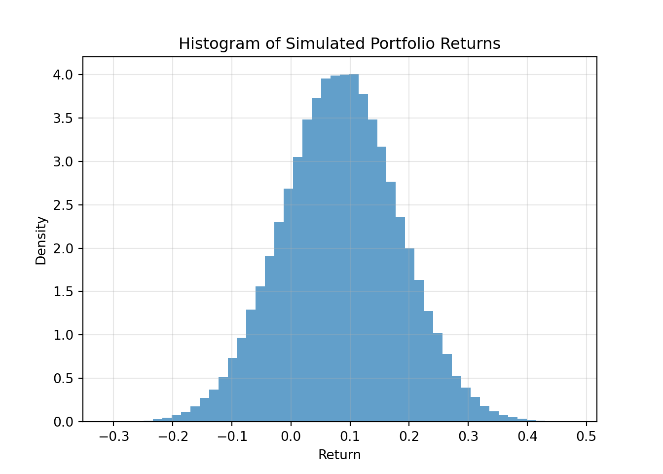

R

# Set seed for reproducibility (optional)
# set.seed(123)

n_sim <- 100000

# Simulate returns for each asset
returns_A <- rnorm(n_sim, mean = 0.10, sd = 0.15)
returns_B <- rnorm(n_sim, mean = 0.06, sd = 0.10)

# Calculate the portfolio return for each simulation
returns_P <- 0.6 * returns_A + 0.4 * returns_B

# Calculate sample mean and variance
mean_P_sim <- mean(returns_P)
var_P_sim <- var(returns_P)

cat("Portfolio Simulation Comparison:\n\n")

Portfolio Simulation Comparison:

cat(sprintf("Theoretical E[Rp] = %.4f, Simulated mean = %.4f\n", 0.084, mean_P_sim))

Theoretical E[Rp] = 0.0840, Simulated mean = 0.0838

cat(sprintf("Theoretical Var(Rp) = %.4f, Simulated variance = %.4f\n\n", 0.0097, var_P_sim))

Theoretical Var(Rp) = 0.0097, Simulated variance = 0.0097

# Bonus: Plot histogram
hist(returns_P, breaks = 50, probability = TRUE, col = rgb(0, 0, 1, 0.7), 
     main = 'Histogram of Simulated Portfolio Returns',
     xlab = 'Return', ylab = 'Density')
grid(col = "gray", lty = "dotted")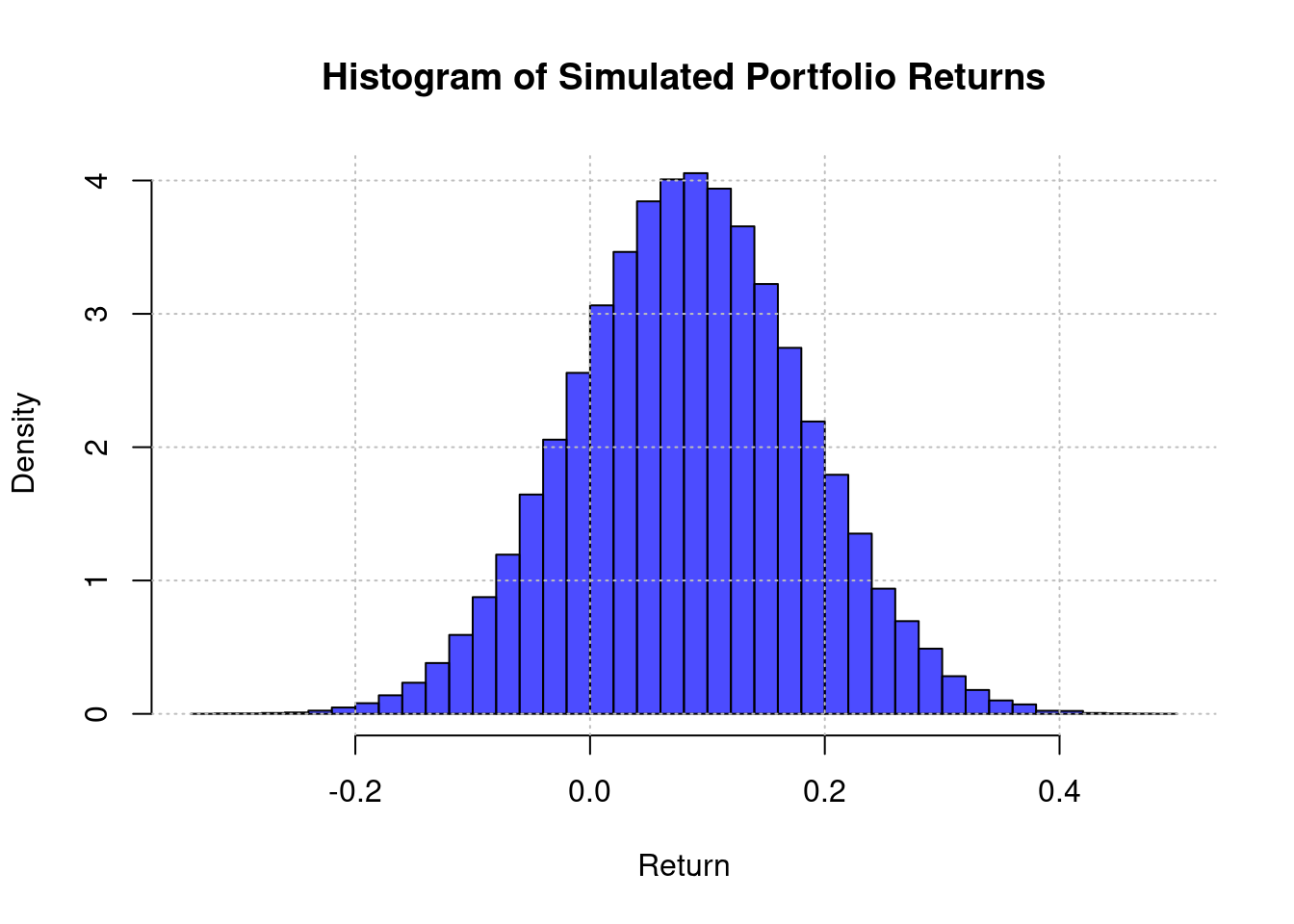

Stata

clear all
set obs 100000
set seed 123  // optional for reproducibility

// Simulate returns for each asset
gen returns_A = rnormal(0.10, 0.15)
gen returns_B = rnormal(0.06, 0.10)

// Calculate the portfolio return
gen returns_P = 0.6 * returns_A + 0.4 * returns_B

// Calculate sample mean and variance
summarize returns_P
scalar mean_P_sim = r(mean)
scalar var_P_sim = r(Var)

// Display results
di "Portfolio Simulation Comparison:" _n
di "Theoretical E[Rp] = 0.0840, Simulated mean = " %6.4f mean_P_sim
di "Theoretical Var(Rp) = 0.0097, Simulated variance = " %6.4f var_P_sim _n

// Bonus: Plot histogram
histogram returns_P, bin(50) frequency normal ///
    title("Histogram of Simulated Portfolio Returns") ///
    xtitle("Return") ytitle("Density")

Rules of Expectation and Variance

Given: \(E[X] = 10, Var(X) = 4, E[Y] = 5, Var(Y) = 9, Cov(X, Y) = -2\).

1. \(E[X + Y]\) \[ E[X + Y] = E[X] + E[Y] = 10 + 5 = 15 \]

2. \(Var(X + Y)\) \[ Var(X + Y) = Var(X) + Var(Y) + 2Cov(X, Y) = 4 + 9 + 2(-2) = 13 - 4 = 9 \]

3. \(E[3X - 2Y]\) \[ E[3X - 2Y] = 3E[X] - 2E[Y] = 3(10) - 2(5) = 30 - 10 = 20 \]

4. \(Var(3X - 2Y)\) \[ Var(3X - 2Y) = 3^2Var(X) + (-2)^2Var(Y) + 2(3)(-2)Cov(X, Y) \] \[ = 9(4) + 4(9) - 12(-2) = 36 + 36 + 24 = 96 \]

5. \(Var(X+Y)\) assuming independence If \(X\) and \(Y\) are independent, \(Cov(X,Y)=0\). \[ Var(X + Y) = Var(X) + Var(Y) = 4 + 9 = 13 \] This variance (13) is higher than the variance when the covariance was -2 (which was 9). The negative covariance implies the variables tend to move in opposite directions, which has a stabilizing (variance-reducing) effect on their sum.

Interpreting Conditional Expectation

(a) Expected income for 12 years of education We substitute \(e=12\) into the formula: \[ E[I | E=12] = 15000 + 4000(12) = 15000 + 48000 = \$63,000 \]

(b) Expected income for 16 years of education We substitute \(e=16\) into the formula: \[ E[I | E=16] = 15000 + 4000(16) = 15000 + 64000 = \$79,000 \]

(c) Is \(E[I|E]\) a number or a random variable? \(E[I|E]\) is a random variable.

Explanation:

• \(E[I|E=e]\) (like in parts a and b) is a single number. It is the expected income for a specific, fixed level of education.
• \(E[I|E]\) (without specifying the value of E) is a function of the random variable \(E\). Since the value of \(E\) (the years of education for a randomly selected person) will vary, the value of \(E[I|E]\) will also vary. Therefore, it is itself a random variable whose outcome depends on the outcome of \(E\).

The Nature of Statistics and Parameters

A parameter is a numerical value that describes a characteristic of an entire population. A statistic is a numerical value that describes a characteristic of a sample. The reason a parameter is considered a fixed value and a statistic is a random variable lies in how they are derived.

• Parameter (Fixed): A parameter is a single, true value. If we could measure the entire population, we would calculate this one value, and it would not change. It’s often unknown in practice (because measuring an entire population is impractical), but it is conceptually a fixed constant.

• Statistic (Random Variable): A statistic is calculated from a subset of the population (a sample). The value of the statistic depends entirely on which specific individuals end up in that random sample. If you were to draw a different random sample, you would get different individuals and thus a different calculated value for the statistic. This variability from sample to sample is what makes a statistic a random variable.

Illustration with Average Height:

• Parameter: The average height of all citizens in a country. There is only one such value. If we could line up every single citizen and measure their height, the average we compute would be the true population mean, \(\mu\). This number is fixed.

• Statistic: The average height of a randomly selected sample of 1,000 citizens.

  • Imagine we take our first sample of 1,000 people and calculate their average height, \(\bar{x}_1 = 175.4\) cm.
  • Now, we discard that sample and draw a new, different random sample of 1,000 people. Maybe this sample, by chance, includes slightly taller people. We calculate their average height and get \(\bar{x}_2 = 176.1\) cm.
  • If we repeat this process again, we might get \(\bar{x}_3 = 175.1\) cm.

The sample mean, \(\bar{x}\), is not fixed. Its value changes depending on the random sample drawn. Therefore, it is a random variable.

Constructing an Exact Sampling Distribution

Given the population [10, 20, 30, 40, 50].

1. Calculate the true population mean, \(\mu\). The population mean is the average of all values in the population. \[ \mu = \frac{10 + 20 + 30 + 40 + 50}{5} = \frac{150}{5} = 30 \]

2. List all possible unique samples of size n=2 without replacement.

There are “5 choose 2” = 10 possible unique samples: 1. (10, 20) 2. (10, 30) 3. (10, 40) 4. (10, 50) 5. (20, 30) 6. (20, 40) 7. (20, 50) 8. (30, 40) 9. (30, 50) 10. (40, 50)

3. Calculate the sample mean (\(\bar{x}\)) for each of these possible samples.

1. mean(10, 20) = 15
2. mean(10, 30) = 20
3. mean(10, 40) = 25
4. mean(10, 50) = 30
5. mean(20, 30) = 25
6. mean(20, 40) = 30
7. mean(20, 50) = 35
8. mean(30, 40) = 35
9. mean(30, 50) = 40
10. mean(40, 50) = 45

4. Present this distribution as a frequency table. This list of all possible sample means constitutes the exact sampling distribution of the sample mean.

Sample Mean (\(\bar{x}\))	Frequency
15	1
20	1
25	2
30	2
35	2
40	1
45	1
Total	10

5. Is the mean of this sampling distribution equal to the true population mean? Let’s calculate the mean of the sampling distribution (the average of all possible sample means): \[ \text{Mean of } \bar{x} = \frac{15(1) + 20(1) + 25(2) + 30(2) + 35(2) + 40(1) + 45(1)}{10} \] \[ = \frac{15 + 20 + 50 + 60 + 70 + 40 + 45}{10} = \frac{300}{10} = 30 \]

Yes, the mean of the sampling distribution (30) is exactly equal to the true population mean (\(\mu=30\)) calculated in part (a). This demonstrates that the sample mean is an unbiased estimator of the population mean.

Simulating a Sampling Distribution

This exercise involves simulating a sampling distribution from a highly skewed Exponential population. A large population of 100,000 data points is drawn from an Exponential distribution with a mean (\(\mu\)) of 10. A histogram of this population data would be highly right-skewed, with most values clustered near zero and a long tail extending to the right.

1. Simulate a population.

2. Draw 5,000 different random samples from this skewed population, each containing n=50 observations.

3. Compute the mean for each of the 5,000 samples, resulting in a list of 5,000 sample means.

4. Plot a histogram of the 5,000 sample means.

Python

import numpy as np
import matplotlib.pyplot as plt

# Set the random seed for reproducibility
np.random.seed(42)

# a) Simulate a population of 100,000 data points from Exponential distribution with mean 10
population_size = 100000
population_mean = 10
population = np.random.exponential(scale=population_mean, size=population_size)

# b) Draw 5,000 different random samples, each with n=50 observations
num_samples = 5000
sample_size = 50
samples = [np.random.choice(population, size=sample_size, replace=False) for _ in range(num_samples)]

# c) Calculate the sample mean for each sample
sample_means = [np.mean(sample) for sample in samples]

# d) Plot a histogram of the 5,000 sample means
plt.figure(figsize=(10, 6))
plt.hist(sample_means, bins=30, edgecolor='black', alpha=0.7)
plt.title('Sampling Distribution of the Mean (n=50)')
plt.xlabel('Sample Mean')
plt.ylabel('Frequency')
plt.grid(True)
plt.show()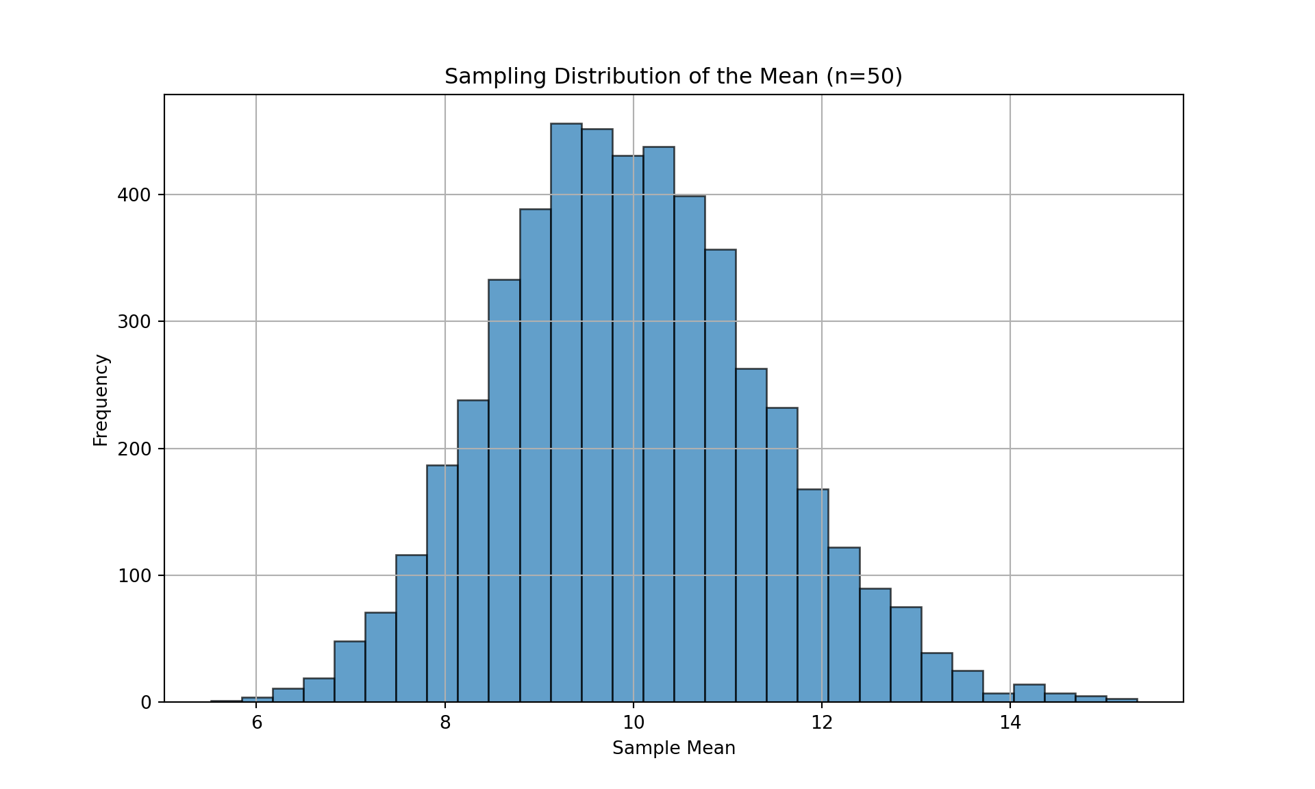

# Print some statistics
print(f"Population mean: {population_mean}")

Population mean: 10

print(f"Mean of sample means: {np.mean(sample_means):.2f}")

Mean of sample means: 9.97

print(f"Standard deviation of sample means: {np.std(sample_means, ddof=1):.2f}")

Standard deviation of sample means: 1.42

R

# Set the random seed for reproducibility
set.seed(42)

# a) Simulate a population of 100,000 data points from Exponential distribution with mean 10
population_size <- 100000
population_mean <- 10
population <- rexp(population_size, rate = 1/population_mean)

# b) Draw 5,000 different random samples, each with n=50 observations
num_samples <- 5000
sample_size <- 50
samples <- lapply(1:num_samples, function(i) sample(population, size = sample_size, replace = FALSE))

# c) Calculate the sample mean for each sample
sample_means <- sapply(samples, mean)

# d) Plot a histogram of the 5,000 sample means
par(mar = c(5, 4, 4, 2) + 0.1) # Adjust margins if needed
hist(sample_means, breaks = 30, col = "lightblue", border = "black", 
     main = "Sampling Distribution of the Mean (n=50)",
     xlab = "Sample Mean", ylab = "Frequency")
grid()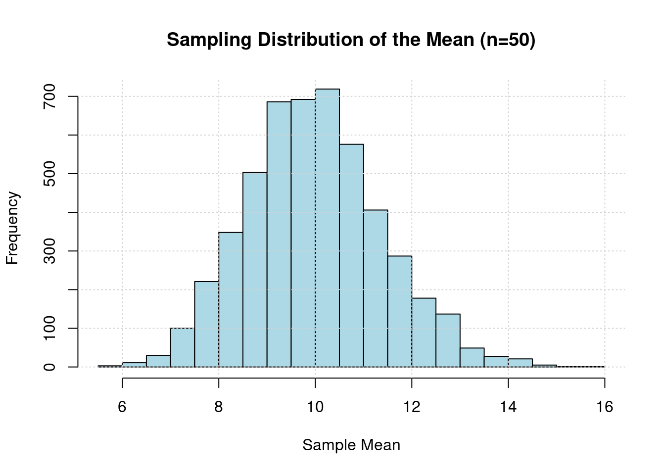

# Print some statistics
cat("Population mean:", population_mean, "\n")

Population mean: 10 

cat("Mean of sample means:", round(mean(sample_means), 2), "\n")

Mean of sample means: 9.99 

cat("Standard deviation of sample means:", round(sd(sample_means), 2), "\n")

Standard deviation of sample means: 1.4 

Stata

clear all
set seed 42

* a) Simulate a population of 100,000 data points from Exponential distribution with mean 10
set obs 100000
scalar population_mean = 10
gen population = -population_mean * ln(1-runiform())

* b) Draw 5,000 different random samples, each with n=50 observations, and calculate their means
local num_samples 5000
local sample_size 50

* Create a matrix to store sample means
matrix sample_means = J(`num_samples', 1, .)

forvalues i = 1/`num_samples' {
    preserve
    * Sample without replacement
    sample `sample_size', count
    * Calculate and store the mean
    quietly summarize population
    matrix sample_means[`i', 1] = r(mean)
    restore
}

* Convert matrix to a variable for analysis
clear
svmat sample_means
rename sample_means1 sample_mean

* d) Plot a histogram of the 5,000 sample means
histogram sample_mean, bin(30) ///
    title("Sampling Distribution of the Mean (n=50)") ///
    xtitle("Sample Mean") ytitle("Frequency") ///
    fcolor("lightblue") lcolor("black")

* Print some statistics
summarize sample_mean
display "Population mean: " population_mean
display "Mean of sample means: " round(r(mean), 0.01)
display "Standard deviation of sample means: " round(r(sd), 0.01)

5. Describe the shape of the histogram of sample means.

Even though the original population has a highly skewed Exponential distribution, the histogram of the 5,000 sample means will look like a Normal distribution. It will be bell-shaped, symmetric, and centered around the true population mean of 10.

This is a direct consequence of the Central Limit Theorem (CLT), which states that for a sufficiently large sample size (n=50 is large enough), the sampling distribution of the sample mean will be approximately normal, regardless of the shape of the original population distribution.

Applying the CLT Conceptually

Given a right-skewed population distribution of package weights with a true mean \(\mu = 8\) kg and a true standard deviation \(\sigma = 5\) kg. A random sample of n=100 is taken.

1. According to the Central Limit Theorem, what can you say about the shape of the sampling distribution of the sample mean weight (\(\bar{x}\))?

Because the sample size n=100 is large (well above the common threshold of 30), the Central Limit Theorem applies. Therefore, the sampling distribution of the sample mean (\(\bar{x}\)) will be approximately Normal, despite the population itself being right-skewed.

2. What will be the theoretical mean of this sampling distribution?

The mean of the sampling distribution of the sample mean is always equal to the population mean. \[ \text{Mean}(\bar{x}) = \mu = 8 \text{ kg} \]

3. What will be the theoretical standard deviation of this sampling distribution (i.e., the standard error)?

The standard deviation of the sampling distribution is called the standard error (SE) and is calculated as \(\sigma / \sqrt{n}\). \[ SE = \frac{\sigma}{\sqrt{n}} = \frac{5}{\sqrt{100}} = \frac{5}{10} = 0.5 \text{ kg} \]

Verifying the CLT in Python/R/Stata

Using the simulation from the Exponential population with true mean \(\mu=10\), true standard deviation \(\sigma=10\), and sample size n=50.

1. From the list of 5,000 sample means you generated, calculate the empirical mean and the empirical standard deviation.

2. According to the CLT, what should the theoretical mean of the sampling distribution be?

The theoretical mean of the sampling distribution is the population mean, \(\mu=10\).

3. According to the CLT, what should the theoretical standard deviation of the sampling distribution (the standard error) be?

The theoretical standard error (SE) is \(\sigma / \sqrt{n}\). \[ \text{Theoretical SE} = \frac{\sigma}{\sqrt{n}} = \frac{10}{\sqrt{50}} \approx \frac{10}{7.071} \approx 1.414 \]

4. Compare the empirical results from part (a) with the theoretical results from parts (b) and (c). Are they close?

Yes, they’re almost equal. This comparison demonstrates how a simulation can empirically verify the predictions of the Central Limit Theorem.

Python

import numpy as np
# Set the random seed for reproducibility (same as before)
np.random.seed(42)

# Parameters
population_size = 100000
population_mean = 10
population_std = 10
num_samples = 5000

population = np.random.exponential(scale=population_mean, size=population_size)

# Sample means
samples = [np.random.choice(population, size=sample_size, replace=False) for _ in range(num_samples)]
sample_means = [np.mean(sample) for sample in samples]

# a) Calculate empirical mean and standard deviation of sample means
empirical_mean = np.mean(sample_means)
empirical_std = np.std(sample_means, ddof=1)  # Using ddof=1 for sample standard deviation
print(f"{empirical_mean:.3f}")

9.975

print(f"{empirical_std:.3f}")

1.420

# c) Theoretical standard error (CLT)
theoretical_se = population_std / np.sqrt(sample_size)
print(f"{theoretical_se:.3f}")

1.414

R

# Set the random seed for reproducibility (same as before)
set.seed(42)

# Parameters
population_size <- 100000
population_mean <- 10  # μ
population_std <- 10
num_samples <- 5000

# Generate population from exponential distribution (assuming this is what you intended)
population <- rexp(population_size, rate = 1/population_mean)  # Exponential with mean = 10

# Sample means
samples <- lapply(1:num_samples, function(x) sample(population, size = sample_size, replace = FALSE))
sample_means <- sapply(samples, mean)

# a) Calculate empirical mean and standard deviation of sample means
empirical_mean <- mean(sample_means)
empirical_std <- sd(sample_means)  # sd() in R uses denominator n-1 by default
print(sprintf("%.3f", empirical_mean))

[1] "9.989"

print(sprintf("%.3f", empirical_std))

[1] "1.402"

# c) Theoretical standard error (CLT)
theoretical_se <- population_std / sqrt(sample_size)
print(sprintf("%.3f", theoretical_se))

[1] "1.414"

Stata

* Set the random seed for reproducibility
set seed 42

* Parameters
local population_size = 100000
local population_mean = 10  // μ
local population_std = 10   // σ (for Exponential distribution, σ = μ)
local sample_size = 50
local num_samples = 5000

* Generate population from exponential distribution
clear
set obs `population_size'
gen population = -`population_mean' * ln(1 - runiform())

* Create variables to store sample means
gen sample_means = .

* Generate sample means
quietly forvalues i = 1/`num_samples' {
    preserve
    sample `sample_size', count
    sum population
    restore
    replace sample_means = r(mean) in `i'
}

* a) Calculate empirical mean and standard deviation of sample means
sum sample_means
local empirical_mean = r(mean)
local empirical_std = r(sd)  // Stata uses denominator n-1 by default
di %6.3f `empirical_mean'
di %6.3f `empirical_std'

* c) Theoretical standard error (CLT)
local theoretical_se = `population_std' / sqrt(`sample_size')
di %6.3f `theoretical_se'

Formulating Hypotheses

• Scenario A: Water Consumption

A city’s water department wants to know if the average daily water consumption per household has changed from last year’s average of 350 gallons.

• Hypotheses:

  • \(H_0: \mu = 350\) (The mean consumption has not changed).
  • \(H_A: \mu \neq 350\) (The mean consumption has changed).

• Test Type: Two-sided test.

• Justification: The keyword is “changed,” which does not specify a direction (increase or decrease). The department is interested in detecting a significant change in either direction.

• Scenario B: New Drug

A pharmaceutical company wants to test if a new drug is effective, meaning it reduces blood pressure compared to a placebo.

• Hypotheses:

  • \(H_0: \mu \ge \mu_{\text{placebo}}\) (The drug does not reduce blood pressure; it has no effect or makes it worse).
  • \(H_A: \mu < \mu_{\text{placebo}}\) (The drug is effective; it reduces blood pressure).

• Test Type: One-sided test (specifically, a left-tailed test).

• Justification: The company is only interested in proving that the drug reduces blood pressure. An outcome where the drug increases blood pressure would lead to the same conclusion as “no effect”: the drug is not marketed. The research question has a clear direction.

• Scenario C: Website Design

An online retailer wants to know if a new website design has a different conversion rate than the old design’s rate of 15%.

• Hypotheses:
  • \(H_0: p = 0.15\) (The new design’s conversion rate is the same as the old one).
  • \(H_A: p \neq 0.15\) (The new design’s conversion rate is different).
• Test Type: Two-sided test.
• Justification: The keyword is “different.” The retailer wants to know if the new design has any impact on the conversion rate, whether it’s an improvement (p > 0.15) or a detriment (p < 0.15). Both outcomes are important for their business decision.

Interpretation and Calculation

Given: n=36, \(\bar{x} = 48.5\) MPG, \(\sigma = 6\) MPG, \(\mu_0 = 50\) MPG, \(\alpha = 0.05\). Test if the true mean is less than 50 MPG.

1. State the null (\(H_0\)) and alternative (\(H_A\)) hypotheses for this test.

• Null Hypothesis (\(H_0\)): The manufacturer’s claim is true. \(H_0: \mu = 50\)
• Alternative Hypothesis (\(H_A\)): The manufacturer’s claim is overstated (the true mean is lower). \(H_A: \mu < 50\)

2. Calculate the standard error of the sample mean. The standard error (SE) is \(\sigma / \sqrt{n}\). \[ SE = \frac{6}{\sqrt{36}} = \frac{6}{6} = 1.0 \text{ MPG} \]

3. Calculate the Z-test statistic.

The Z-statistic measures how many standard errors the sample mean is from the hypothesized population mean. \[ Z = \frac{\bar{x} - \mu_0}{SE} = \frac{48.5 - 50}{1.0} = -1.5 \]

4. Using your Z-statistic, find the corresponding p-value. Since this is a left-tailed test (\(H_A: \mu < 50\)), the p-value is the area under the standard normal curve to the left of Z = -1.5. Using a Z-table or statistical software, we find: \[ p\text{-value} = P(Z \le -1.5) \approx 0.0668 \]

5. Based on your p-value and the significance level of \(\alpha=0.05\), what is your conclusion?

We compare the p-value to the significance level \(\alpha\). * p-value (0.0668) > \(\alpha\) (0.05)

Since the p-value is greater than the significance level, we fail to reject the null hypothesis.

Conclusion: At the 5% significance level, there is insufficient statistical evidence to conclude that the true mean fuel efficiency of the new hybrid model is less than 50 MPG. The consumer watchdog group does not have strong enough evidence to refute the manufacturer’s claim.

Performing a Hypothesis Test

Use the WAGE2.DTA dataset. Import it in R/Python/Stata. Conduct a hypothesis test on the IQ variable. The null hypothesis is that mu_0 = 100.

1. Calculate the standard error and the Z-test statistic in Python.

2. The p-value for a two-tailed test is the area under the standard normal curve that is more extreme (on both sides) than your calculated Z-statistic. Use scipy.stats.norm.cdf() or pnorm() to find this p-value.

Python

import pandas as pd
import numpy as np
from scipy.stats import norm

np.random.seed(42)
url = 'https://raw.githubusercontent.com/basm92/ee_website/refs/heads/master/tutorials/datafiles/WAGE2.DTA'
data = pd.read_stata(url)
mu_0 = 100

# a)  Calculate the standard error and the Z-test statistic in Python.
sigma = np.std(data['IQ'])
n = len(data['IQ'])

se = sigma / np.sqrt(n)
sample_mean = np.mean(data['IQ'])
z = (sample_mean - mu_0) / se

# b)  The p-value for a two-tailed test is the area under the standard normal curve that is more extreme (on both sides) than your calculated Z-statistic. Use `scipy.stats.norm.cdf()` or `pnorm()` to find this p-value.
p_value = (1 - norm.cdf(z)) + norm.cdf(-z)
print(f"The p-value is: {p_value:.3f}")

# Meaning we reject the null hypothesis that the average IQ in the population is 100.

R

# Load required packages
library(haven)
library(dplyr)

set.seed(42)
data <- read_dta("https://raw.githubusercontent.com/basm92/ee_website/refs/heads/master/tutorials/datafiles/WAGE2.DTA")
mu_0 <- 100

# a) Calculate the standard error and the Z-test statistic in R
sigma <- sd(data$IQ)
n <- length(data$IQ)

se <- sigma / sqrt(n)
sample_mean <- mean(data$IQ)
z <- (sample_mean - mu_0) / se

# b) The p-value for a two-tailed test
p_value <- (1 - pnorm(z)) + pnorm(-z)
cat(sprintf("The p-value is: %.3f\n", p_value))

The p-value is: 0.009

# Meaning we reject the null hypothesis that the average IQ in the population is 100.

Stata

* Set random seed for reproducibility
set seed 42

* Load the data
use "https://raw.githubusercontent.com/basm92/ee_website/refs/heads/master/tutorials/datafiles/WAGE2.DTA", clear

* Set null hypothesis value
scalar mu_0 = 100

* a) Calculate standard error and Z-test statistic
quietly summarize IQ
scalar sigma = r(sd)
scalar n = r(N)

scalar se = sigma / sqrt(n)
scalar sample_mean = r(mean)
scalar z = (sample_mean - mu_0) / se

* b) Calculate two-tailed p-value
scalar p_value = 2 * (1 - normal(abs(z)))  // Two-tailed p-value

* Display results
di "The p-value is: " %6.3f p_value

* Meaning we reject the null hypothesis that the average IQ in the population is 100.

Correct Interpretation

Given a 95% confidence interval for average study hours: [12.5, 15.0].

The correct interpretation is Statement 2.

• Statement 2 (Correct): “We are 95% confident that the method we used to generate this interval captures the true average study time for all students at the university.”

• Explanation: This statement is correct because it properly places the “confidence” (which is related to probability) on the method, not on the true parameter. The true population mean (\(\mu\)) is a fixed, unknown number. It does not vary. What is random is our sampling process. If we were to repeat our sampling procedure 100 times, we would generate 100 different confidence intervals. The “95% confidence” means we expect about 95 of those 100 intervals to successfully “capture” or contain the true, fixed population mean. Our specific interval, [12.5, 15.0], is just one of those results.

• Statement 1 (Incorrect): “There is a 95% probability that the true average study time for all students at the university is between 12.5 and 15.0 hours.”

• Explanation of Error: This statement is a very common misinterpretation. It incorrectly implies that the true mean \(\mu\) is a random variable that has a 95% chance of falling within our calculated interval. But \(\mu\) is fixed. Once we have calculated our interval [12.5, 15.0], the true mean \(\mu\) is either inside this specific range or it is not. The probability is either 1 or 0, we just don’t know which. The 95% refers to the long-run success rate of the procedure used to create the interval.

Factors Affecting Interval Width

The width of a confidence interval is determined by the Margin of Error: Width = 2 * (Critical Value) * (Standard Error).

1. Increasing the confidence level from 90% to 99%.

This will make the confidence interval wider. To be more confident that you have captured the true mean, you need to use a larger critical value (e.g., Z for 99% is ~2.576 vs. ~1.645 for 90%). A larger critical value increases the margin of error, thus widening the interval. Think of it as needing a wider net to be more sure of catching the fish.

2. Increasing the sample size from 100 to 400.

This will make the confidence interval narrower. The sample size (n) is in the denominator of the standard error (\(\sigma/\sqrt{n}\)). Increasing n decreases the standard error. A smaller standard error results in a smaller margin of error and a more precise, narrower interval. More data provides a more accurate estimate.

3. The sample having a larger standard deviation.

This will make the confidence interval wider. The standard deviation (\(\sigma\)) is in the numerator of the standard error. A larger standard deviation indicates that the data points in the population are more spread out and variable. This increased variability leads to a larger standard error, a larger margin of error, and thus a wider interval to account for the greater uncertainty.

Constructing a Confidence Interval

Given: n=36, \(\bar{x} = 48.5\) MPG, \(\sigma = 6\) MPG.

1. Calculate a 95% confidence interval for the true mean fuel efficiency.

2. Now, calculate a 99% confidence interval using the same data.

Python

import numpy as np
from scipy.stats import norm

# a)  Calculate a 95% confidence interval for the true mean fuel efficiency.
# Given data
x_bar = 48.5  # Sample mean
sigma = 6     # Population standard deviation
n = 36        # Sample size
confidence_level = 0.95

# 1. Point estimate is the sample mean
point_estimate = x_bar

# 2. Calculate the standard error
standard_error = sigma / np.sqrt(n)

# 3. Find the critical Z-value for a 95% CI
# We need to leave (1 - 0.95)/2 = 0.025 in each tail.
# So we look for the Z-value at the 0.975 percentile.
critical_value = norm.ppf(1 - (1 - confidence_level) / 2) # Equivalent to norm.ppf(0.975)

# 4. Calculate the margin of error
margin_of_error = critical_value * standard_error

# 5. Construct the interval
lower_bound = point_estimate - margin_of_error
upper_bound = point_estimate + margin_of_error

print(f"Point Estimate: {point_estimate}")

Point Estimate: 48.5

print(f"Standard Error: {standard_error:.2f}")

Standard Error: 1.00

print(f"Critical Z-value: {critical_value:.3f}")

Critical Z-value: 1.960

print(f"Margin of Error: {margin_of_error:.3f}")

Margin of Error: 1.960

print(f"95% Confidence Interval: [{lower_bound:.3f}, {upper_bound:.3f}]")

95% Confidence Interval: [46.540, 50.460]

# b) We only need to change the confidence level and find the new critical value.
critical_value = norm.ppf(0.995)
margin_of_error = critical_value * standard_error
lower_bound = x_bar - margin_of_error
upper_bound = x_bar + margin_of_error
print(f"Critical Z-value: {critical_value:.3f}")

Critical Z-value: 2.576

print(f"Margin of Error: {margin_of_error:.3f}")

Margin of Error: 2.576

print(f"95% Confidence Interval: [{lower_bound:.3f},{upper_bound:.3f}]")

95% Confidence Interval: [45.924,51.076]

R

# a) Calculate a 95% confidence interval for the true mean fuel efficiency.
# Given data
x_bar <- 48.5  # Sample mean
sigma <- 6     # Population standard deviation
n <- 36        # Sample size
confidence_level <- 0.95

# 1. Point estimate is the sample mean
point_estimate <- x_bar

# 2. Calculate the standard error
standard_error <- sigma / sqrt(n)

# 3. Find the critical Z-value for a 95% CI
# We need to leave (1 - 0.95)/2 = 0.025 in each tail.
# So we look for the Z-value at the 0.975 percentile.
critical_value <- qnorm(1 - (1 - confidence_level) / 2) # Equivalent to qnorm(0.975)

# 4. Calculate the margin of error
margin_of_error <- critical_value * standard_error

# 5. Construct the interval
lower_bound <- point_estimate - margin_of_error
upper_bound <- point_estimate + margin_of_error

cat("Point Estimate:", point_estimate, "\n")

Point Estimate: 48.5 

cat(sprintf("Standard Error: %.2f\n", standard_error))

Standard Error: 1.00

cat(sprintf("Critical Z-value: %.3f\n", critical_value))

Critical Z-value: 1.960

cat(sprintf("Margin of Error: %.3f\n", margin_of_error))

Margin of Error: 1.960

cat(sprintf("95%% Confidence Interval: [%.3f, %.3f]\n", lower_bound, upper_bound))

95% Confidence Interval: [46.540, 50.460]

# b) We only need to change the confidence level and find the new critical value.
critical_value <- qnorm(0.995)
margin_of_error <- critical_value * standard_error
lower_bound <- x_bar - margin_of_error
upper_bound <- x_bar + margin_of_error
cat(sprintf("Critical Z-value: %.3f\n", critical_value))

Critical Z-value: 2.576

cat(sprintf("Margin of Error: %.3f\n", margin_of_error))

Margin of Error: 2.576

cat(sprintf("95%% Confidence Interval: [%.3f, %.3f]\n", lower_bound, upper_bound))

95% Confidence Interval: [45.924, 51.076]

Stata

* a) Calculate a 95% confidence interval for the true mean fuel efficiency.
* Given data
scalar x_bar = 48.5  // Sample mean
scalar sigma = 6     // Population standard deviation
scalar n = 36        // Sample size
scalar confidence_level = 0.95

* 1. Point estimate is the sample mean
scalar point_estimate = x_bar

* 2. Calculate the standard error
scalar standard_error = sigma / sqrt(n)

* 3. Find the critical Z-value for a 95% CI
* We need to leave (1 - 0.95)/2 = 0.025 in each tail.
* So we look for the Z-value at the 0.975 percentile.
scalar critical_value = invnormal(1 - (1 - confidence_level)/2) // Equivalent to invnormal(0.975)

* 4. Calculate the margin of error
scalar margin_of_error = critical_value * standard_error

* 5. Construct the interval
scalar lower_bound = point_estimate - margin_of_error
scalar upper_bound = point_estimate + margin_of_error

di "Point Estimate: " point_estimate
di "Standard Error: " %4.2f standard_error
di "Critical Z-value: " %4.3f critical_value
di "Margin of Error: " %4.3f margin_of_error
di "95% Confidence Interval: [" %4.3f lower_bound ", " %4.3f upper_bound "]"

* b) We only need to change the confidence level and find the new critical value.
scalar critical_value = invnormal(0.995)
scalar margin_of_error = critical_value * standard_error
scalar lower_bound = x_bar - margin_of_error
scalar upper_bound = x_bar + margin_of_error
di "Critical Z-value: " %4.3f critical_value
di "Margin of Error: " %4.3f margin_of_error
di "95% Confidence Interval: [" %4.3f lower_bound ", " %4.3f upper_bound "]"

As expected, the 99% confidence interval is wider than the 95% confidence interval. This is because we require a wider range to be more confident that it contains the true population mean.