The practical interpretation of this coefficient is as follows: holding the square footage (sqrft) and the number of bedrooms (bdrms) constant, for every one-unit increase in the size of the land plot (in square feet), the predicted price of the house is expected to increase by 0.002 units. Since the price is likely measured in thousands of dollars (a common practice in such datasets), this would mean an increase of 2 dollars for every additional square foot of lot size. For example, an increase of 1,000 square feet in lot size is associated with a 2,000 dollar increase in the predicted price of the house, all else being equal.
In model (2), the coefficient for the colonial variable is 13.078. However, the p-value associated with this coefficient is greater than 0.1, indicating that it is not statistically significant at conventional levels. The interpretation of this is that, while the model estimates that a colonial-style house is associated with a 13,078 dollars higher price than a non-colonial style house (holding sqrft and bdrms constant), this effect is not statistically significant. This means that we cannot confidently conclude that there is a real relationship between a house being colonial style and its price in the population from which this data was sampled. The observed difference in price could very well be due to random chance or sampling variability. Therefore, based on this model, there is insufficient evidence to claim that the colonial style of a house has a meaningful impact on its sale price.
Wage Determinants
Estimate a multiple linear regression model where lhrwage is the dependent variable and educ, exper, union, and male are the independent variables.
Present the summary of your regression model, including the estimated coefficients, standard errors, t-statistics, and p-values.
Based on your regression output, provide a clear and concise interpretation for the educ and union coefficients.
An additional year of educ is associated with a 7.8% increase in the hourly wage, everything else equal. Union members have a 13% higher hourly wage than non-union members, everything else equal.
Perform a hypothesis test for the exper coefficient to determine if it is statistically significant at the 5% significance level. State your null and alternative hypotheses, report the relevant test statistic and p-value from your model output, and conclude whether you reject or fail to reject the null hypothesis. What does this conclusion imply about the relationship between experience and the logarithm of hourly wage in this model?
\(H_0: \beta_\text{exper}=0\). \(H_A: \beta_\text{exper}\neq 0\). \(t=3.774\) and the \(p\)-value is 0. That means that observing a test statistic such as the one we actually observe is extremely unlikely under the null hypothesis. Therefore we reject the null hypothesis of a \(\beta\)-coefficient of 0. We thus think there is a non-zero relationship between experience and the log of the hourly wage.
# 1. Estimate a multiple linear regression model where `lhrwage` is the dependent variable and `educ`, `exper`, `union`, and `male` are the independent variables.import pyfixest as pfimport pandas as pdwages = pd.read_stata("../tutorials/datafiles/SLEEP75.DTA")model = pf.feols("lhrwage ~ educ + exper + union + male", data=wages)# 2. Present the summary of your regression model, including the estimated coefficients, standard errors, t-statistics, and p-values.model.summary()
# 1. Estimate a multiple linear regression model where `lhrwage` is the dependent variable and `educ`, `exper`, `union`, and `male` are the independent variables.library(haven); library(fixest)wages <-read_dta("../tutorials/datafiles/SLEEP75.DTA")model <-feols(lhrwage ~ educ + exper + union + male, data = wages)# 2. Present the summary of your regression model, including the estimated coefficients, standard errors, t-statistics, and p-values.summary(model)
use https://github.com/basm92/ee_website/raw/refs/heads/master/tutorials/datafiles/SLEEP75.DTA, clear// Run the regression and display full resultsreg lhrwage educ exper union male
Heteroskedasticity
After estimating the OLS model, obtain the residuals.1
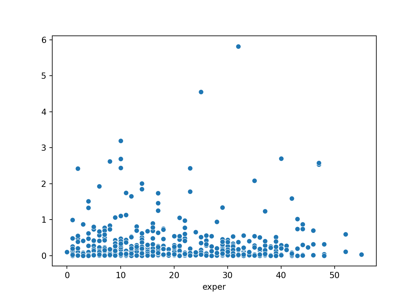
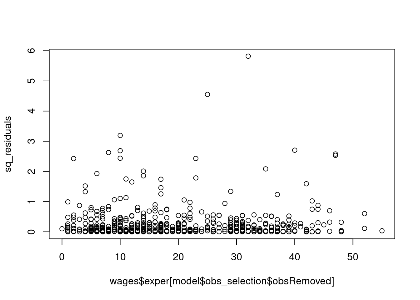
Create a scatter plot with the values of exper on the x-axis and the squared residuals on the y-axis.
Examine the plot. Does the spread of the squared residuals appear to change as the fitted values decrease? Describe the pattern you see and explain why it might suggest the presence of heteroskedasticity.
Re-estimate the model, but this time calculate heteroskedasticity-robust standard errors.
Compare the “normal” OLS standard errors with the robust standard errors for each of the four coefficients (educ, exper, union, and male).
# 1. After estimating the OLS model, obtain the residuals.^[In R, you can use the `model$residuals`. In Python, it's `model.resid()`. In Stata, it's `predict res, residuals`. ]import seaborn as snsimport matplotlib.pyplot as pltsq_residuals = model.resid()**2# 2. Create a scatter plot with the values of `educ` on the x-axis and the squared residuals on the y-axis.sns.scatterplot(x=model._data['exper'], y=sq_residuals)plt.show()
# 4. Re-estimate the model, but this time calculate **heteroskedasticity-robust standard errors**.
model.vcov('HC1').summary()
library(ggplot2)# 1. After estimating the OLS model, obtain the residuals.^[In R, you can use the `model$residuals`. In Python, it's `model.resid()`. In Stata, it's `predict res, residuals`. ]sq_residuals <- model$residuals^2# 2. Create a scatter plot with the values of `educ` on the x-axis and the squared residuals on the y-axis.plot(x=wages$exper[model$obs_selection$obsRemoved], y=sq_residuals)
# 4. Re-estimate the model, but this time calculate **heteroskedasticity-robust standard errors**. model_hc <-feols(lhrwage ~ educ + exper + union + male, data = wages, vcov='hc1')summary(model_hc)
* 1. After estimating the OLS model, obtain the residuals.^[In R, you can use the `model$residuals`. In Python, it's `model.resid()`. In Stata, it's `predict res, residuals`. ]reg lhrwage educ exper union malepredict residuals, residualsgen sq_residuals = residuals^2* 2. Create a scatter plot with the valuesof `educ` on the x-axis and the squared residuals on the y-axis.scatter sq_residuals exper, title("Squared Residuals vs Experience") xtitle("Experience") ytitle("Squared Residuals")* 3. Re-estimate model with heteroskedasticity-robust standard errorsreg lhrwage educ exper union male, robust
Show that the expected value of the estimator from the incorrect short regression is\(E(\hat{\gamma}_1) = \beta_1 + \beta_2 \cdot \delta_1\).
The estimated coefficient from the incorrect (short) regression of \(y\) on \(x_1\) is: \[ \hat{\gamma}_1 = \frac{\sum(x_{1i}-\bar{x}_1)y_i}{\sum(x_{1i}-\bar{x}_1)^2} \]
Substitute the true population model for \(y_i\): \(y_i = \beta_0 + \beta_1 x_{1i} + \beta_2 x_{2i} + u_i\). \[ \hat{\gamma}_1 = \frac{\sum(x_{1i}-\bar{x}_1)(\beta_0 + \beta_1 x_{1i} + \beta_2 x_{2i} + u_i)}{\sum(x_{1i}-\bar{x}_1)^2} \]
Distribute the numerator and separate the terms, just as in the unbiasedness proof: \[ \hat{\gamma}_1 = \frac{\sum(x_{1i}-\bar{x}_1)\beta_0}{\sum(x_{1i}-\bar{x}_1)^2} + \frac{\sum(x_{1i}-\bar{x}_1)\beta_1 x_{1i}}{\sum(x_{1i}-\bar{x}_1)^2} + \frac{\sum(x_{1i}-\bar{x}_1)\beta_2 x_{2i}}{\sum(x_{1i}-\bar{x}_1)^2} + \frac{\sum(x_{1i}-\bar{x}_1)u_i}{\sum(x_{1i}-\bar{x}_1)^2} \]
Simplify each term:
The first term is 0. (Covariance with a constant)
The second term simplifies to \(\beta_1\).
The third term can be rewritten as \(\beta_2 \left( \frac{\sum(x_{1i}-\bar{x}_1)x_{2i}}{\sum(x_{1i}-\bar{x}_1)^2} \right)\).
The fourth term remains. So, \[ \hat{\gamma}_1 = \beta_1 + \beta_2 \left( \frac{\sum(x_{1i}-\bar{x}_1)(x_{2i}-\bar{x}_2)}{\sum(x_{1i}-\bar{x}_1)^2} \right) + \frac{\sum(x_{1i}-\bar{x}_1)u_i}{\sum(x_{1i}-\bar{x}_1)^2} \](Note: We can replace\(x_{2i}\) with \((x_{2i}-\bar{x}_2)\) in the numerator because \(\sum(x_{1i}-\bar{x}_1)\bar{x}_2=0\).)
Recognize that the term in the parenthesis is the formula for the OLS slope coefficient from a regression of \(x_2\) on \(x_1\). Let’s call this \(\hat{\delta}_1\). \[ \hat{\delta}_1 = \frac{\text{Cov}(x_1, x_2)}{\text{Var}(x_1)} = \frac{\sum(x_{1i}-\bar{x}_1)(x_{2i}-\bar{x}_2)}{\sum(x_{1i}-\bar{x}_1)^2} \] The equation becomes: \(\hat{\gamma}_1 = \beta_1 + \beta_2 \hat{\delta}_1 + \text{error term involving u}\).
Now, take the expectation. We assume that in the population, the relationship between \(x_2\) and \(x_1\) is \(E(x_2|x_1) = \delta_0 + \delta_1 x_1\). So \(E(\hat{\delta}_1) = \delta_1\). \[ E(\hat{\gamma}_1) = E(\beta_1) + E(\beta_2 \hat{\delta}_1) + E(\text{error term}) \]\[ E(\hat{\gamma}_1) = \beta_1 + \beta_2 E(\hat{\delta}_1) + 0 \quad (\text{since } E(u|X)=0) \]\[ E(\hat{\gamma}_1) = \beta_1 + \beta_2 \delta_1 \] The term \(\beta_2 \delta_1\) is the omitted variable bias.
Perfect Multicollinearity
(a) What does it mean for\(x_1\) and \(x_2\) to have perfect multicollinearity?
Perfect multicollinearity means that one explanatory variable is a perfect linear function of another. For example, \(x_1 = c_0 + c_1 x_2\) for some constants \(c_0\) and \(c_1\) where \(c_1 \neq 0\). This means there is no independent variation in \(x_1\) that is not associated with \(x_2\). A common example is including a variable in different units (e.g., height in meters and height in centimeters) in the same regression.
(b) Analytically, what happens to the value of\(R_1^2\) under perfect multicollinearity?
\(R_1^2\) is the R-squared from a regression of \(x_1\) on \(x_2\). If \(x_1\) is a perfect linear function of \(x_2\), then the regression of \(x_1\) on \(x_2\) will explain 100% of the variation in \(x_1\). Therefore, \(R_1^2 = 1\).
(c) Explain mathematically why it is impossible to calculate\(\hat{\beta}_1\).
The variance of the OLS estimator \(\hat{\beta}_1\) is given by: \[ Var(\hat{\beta}_1) = \frac{\sigma^2}{SST_1 (1 - R_1^2)} \]
Under perfect multicollinearity, we established that \(R_1^2 = 1\). Substituting this into the denominator: \[ \text{Denominator} = SST_1 (1 - 1) = SST_1 \cdot 0 = 0 \]
The variance of the estimator becomes: \[ Var(\hat{\beta}_1) = \frac{\sigma^2}{0} \rightarrow \infty \]
Since the variance of the estimator is infinite, the OLS estimator is undefined. The OLS procedure fails because it is mathematically impossible to distinguish the unique effect of \(x_1\) from the effect of \(x_2\) when they are perfectly linearly related.
Zero Conditional Mean
(a) Explain in your own words what this assumption means.
The Zero Conditional Mean assumption, \(E(u|x) = 0\), means that the average value of all unobserved factors (the error term, \(u\)) is zero for any given value of the explanatory variable (\(x\)). Put simply, it means that the unobserved factors are not systematically related to, or correlated with, the explanatory variable.
(b) Using wage on education, explain why “innate ability” violates this assumption.
In a model \(\text{wage} = \beta_0 + \beta_1 \text{education} + u\), “innate ability” is an unobserved factor and is therefore part of the error term \(u\).
It is very likely that innate ability is correlated with both wage and education.
People with higher ability may earn higher wages regardless of their education level.
People with higher ability may find it easier to succeed in school and are therefore more likely to attain higher levels of education.
Because ability is in u and is also correlated with education, the average level of u is not zero across different levels of education. Specifically, \(E(u|\text{education})\) will be higher for higher levels of education. This violates the Zero Conditional Mean assumption.
(c) In which direction will\(\hat{\beta}_1\) be biased?
The bias will be positive. The OLS estimate \(\hat{\beta}_1\) will be overstated.
Reasoning (using the OVB formula): The bias is \(\beta_2 \cdot \delta_1\).
\(\beta_2\) is the effect of the omitted variable (ability) on the outcome (wage). This effect is positive (\(\beta_2 > 0\)).
\(\delta_1\) is the correlation between the included variable (education) and the omitted variable (ability). This correlation is also positive (\(\delta_1 > 0\)).
Since the bias term is the product of two positive numbers, the bias is positive. The OLS estimate \(\hat{\beta}_1\) will mistakenly attribute some of the wage-increasing effect of ability to education, leading to an estimate that is larger than the true causal effect of education on wages.
Mitigating Omitted Variable Bias
What are two or three other variables you would want to include in the wage on education model? What are the practical challenges?
Variables to Include:
Cognitive Ability / IQ: To control for the “innate ability” bias discussed earlier.
Quality of Institution: The return to a degree from a top university is likely higher than from a less selective one. This could be measured by university ranking or average test scores of admitted students.
Parental Background: Variables like parents’ education and income can capture family network effects, financial support, and environmental factors that influence both a child’s education and future earnings.
Practical Challenges:
Data Availability: Most standard economic datasets (like labor force surveys) do not collect information on IQ, school quality, or detailed parental background.
Measurement: These variables are difficult to measure accurately. “Ability” is a complex construct, and IQ tests are controversial. “School quality” is also multifaceted and hard to summarize with a single number.
Privacy: Data on IQ and parental income are highly sensitive and can be difficult to obtain due to privacy concerns.
Hypothesis Testing
t-test for exper:
Hypotheses:
Null Hypothesis (\(H_0\)): \(\beta_{exper} = 0\). Work experience has no effect on wage, holding education constant.
Alternative Hypothesis (\(H_A\)): \(\beta_{exper} \neq 0\). Work experience has a non-zero effect on wage, holding education constant.
Conclusion: Yes, you would reject the null hypothesis at a 5% significance level. The p-value for exper is < 0.001, which is much smaller than the significance level of 0.05. This indicates that the estimated effect of experience is statistically significant.
F-test for Overall Significance:
Hypotheses:
Null Hypothesis (\(H_0\)): \(\beta_{educ} = 0 \text{ and } \beta_{exper} = 0\). Neither education nor experience have an effect on wages; the model has no explanatory power.
Alternative Hypothesis (\(H_A\)): At least one of the coefficients (\(\beta_{educ}\) or \(\beta_{exper}\)) is not equal to zero.
Conclusion: The p-value for the F-test is < 0.001. This means we reject the null hypothesis and conclude that the model as a whole is statistically significant. The variables educ and exper are jointly significant in explaining the variation in wage.
Restricted Model for the Joint Hypothesis Test:
Regression Equation: If we impose the restriction that \(\beta_1=0\) and \(\beta_2=0\), the regression equation becomes: \[
\text{wage} = \beta_0 + u
\] This model suggests that the best prediction for anyone’s wage, regardless of their education or experience, is simply the average wage (\(\hat{\beta}_0 = \bar{\text{wage}}\)).
Sum of Squared Residuals (\(SSR_{restricted}\)): In this restricted model, the residuals are the differences between each observation and the sample mean (\(u_i = y_i - \bar{y}\)). The Sum of Squared Residuals is therefore the sum of the squared deviations from the mean, which is the definition of the Total Sum of Squares (TSS). Using the provided statistics, we can calculate it: \[
R^2 = 1 - \frac{SSR_{unrestricted}}{TSS} \implies TSS = \frac{SSR_{unrestricted}}{1 - R^2}
\]\[
SSR_{restricted} = TSS = \frac{875.2}{1 - 0.583} = \frac{875.2}{0.417} \approx 2098.8
\]
Interpreting Interaction Effects
Equation for Non-Homeowners: For non-homeowners, is_homeowner = 0. We substitute this into the equation: \[
\widehat{\text{donations}} = 50 + 150(0) + 5 \cdot \text{age} + 3(0 \cdot \text{age})
\]\[
\widehat{\text{donations}} = 50 + 5 \cdot \text{age}
\] The estimated effect of an additional year of age on donations for a non-homeowner is €5.
Equation for Homeowners: For homeowners, is_homeowner = 1. We substitute this into the equation and group terms: \[
\widehat{\text{donations}} = 50 + 150(1) + 5 \cdot \text{age} + 3(1 \cdot \text{age})
\]\[
\widehat{\text{donations}} = (50 + 150) + (5 + 3) \cdot \text{age}
\]\[
\widehat{\text{donations}} = 200 + 8 \cdot \text{age}
\] The estimated effect of an additional year of age on donations for a homeowner is €8.
Interpretation of the Interaction Coefficient: The coefficient on the interaction term (\(\hat{\beta}_3 = 3\)) represents the difference in the slopes between the two groups. It means that the positive effect of an additional year of age on charitable donations is €3 higher for homeowners than it is for non-homeowners.
Predicted Difference at Age 50:
Predicted donations for a 50-year-old homeowner: \(200 + 8(50) = 200 + 400 = 600\).
Predicted donations for a 50-year-old non-homeowner: \(50 + 5(50) = 50 + 250 = 300\).
The predicted difference is \(600 - 300 = \text{€}300\).
Good vs. Bad Controls
fitness_level (before training): Good Control (Confounder).
Justification: This is a pre-treatment variable. It is likely correlated with the treatment (fitter people are more likely to run a marathon) and the outcome (fitter people may be happier in general). Failing to control for it would likely lead to omitted variable bias, where the marathon’s effect would incorrectly absorb the pre-existing effect of fitness.
hours_trained: Bad Control (Mediator).
Justification: Training is a direct consequence of the decision to run a marathon and lies on the causal pathway between running the marathon and happiness. Controlling for it would mean you are holding constant one of the key mechanisms through which running a marathon affects happiness. This would “block” part of the effect you want to measure.
has_gym_membership (after the marathon): Bad Control (Collider).
Justification: This variable is a common effect of both the treatment (ran_marathon) and the outcome (happiness). Running a marathon might make someone feel accomplished and buy a membership, and being happy might also make someone more likely to buy a membership. Controlling for a variable that is caused by both the treatment and the outcome will induce a spurious correlation and bias your estimate of the causal effect.
Correct Standard Errors
Study A:(b) Heteroskedasticity-Robust (HC) SEs.
Explanation: The suspicion that the variance of electricity usage is different for high-income and low-income households is a direct description of heteroskedasticity. Since the data is a cross-section of households, HC-robust standard errors are the appropriate tool to ensure valid statistical inference.
Study B:(c) Cluster-Robust SEs, clustered at the country level.
Explanation: This is panel data where observations for the same country over time are likely correlated due to persistent unobserved factors (e.g., policy, geography, culture). This violates the assumption of independent errors. Clustering the standard errors by country allows the errors for a given country to be correlated over time, leading to more accurate inference.
Study C:(c) Cluster-Robust SEs, clustered at the school level.
Explanation: Students within the same school share common unobserved factors (teacher quality, school resources, peer effects). This will likely cause the error terms for students in the same school to be correlated. To account for this intra-cluster correlation, one must cluster the standard errors at the school level.
Footnotes
In R, you can use the model$residuals. In Python, it’s model.resid(). In Stata, it’s predict res, residuals. ↩︎