To estimate the fixed effects model in R, you use the plm function from the plm package. You need to specify the formula, the dataset, the individual and time identifiers in the index argument, and set model = "within" for the fixed effects estimator.
# Load the required libraries and datalibrary(wooldridge)library(tidyverse, quietly=TRUE)library(plm)url <-"https://raw.githubusercontent.com/basm92/ee_website/refs/heads/master/tutorials/datafiles/jtrain.csv"jtrain <-read_csv2(url)# Estimate the firm-level fixed effects model# index = c("fcode", "year") tells plm that 'fcode' is the individual (firm) ID# and 'year' is the time variable.fe_model <-plm(scrap ~ grant, data = jtrain,index =c("fcode", "year"), model ="within")# Print the summary to see the resultssummary(fe_model)
Oneway (individual) effect Within Model

Call:
plm(formula = scrap ~ grant, data = jtrain, model = "within",
    index = c("fcode", "year"))

Balanced Panel: n = 54, T = 3, N = 162

Residuals:
       Min.     1st Qu.      Median     3rd Qu.        Max.
-10.4000000  -0.2511494  -0.0033333   0.2000000  10.2000000

Coefficients:
      Estimate Std. Error t-value Pr(>|t|)
grant -0.75345    0.48230 -1.5622   0.1212

Total Sum of Squares:    492.17
Residual Sum of Squares: 481.19
R-Squared:      0.0223
Adj. R-Squared: -0.47112
F-statistic: 2.44049 on 1 and 107 DF, p-value: 0.12119
To estimate the fixed effects model in Python, you use the feols function from the pyfixest package. You need to specify the formula and the individual fixed effects in the formula for the fixed effects estimator.
import pandas as pdimport pyfixest as pfurl ="https://raw.githubusercontent.com/basm92/ee_website/refs/heads/master/tutorials/datafiles/jtrain.csv"jtrain = pd.read_csv(url, sep=";", decimal=',')fit = pf.feols(fml="scrap ~ grant | fcode", data=jtrain)# fixed effects separated from the ind. vars. by | fit.vcov('iid').summary()
* 1. Clear any existing datainmemoryclear* 2. Import the data directly from the URL* We specify the delimiter as a semicolon (;) and the decimal as a comma (,)import delimited "https://raw.githubusercontent.com/basm92/ee_website/refs/heads/master/tutorials/datafiles/jtrain.csv", delimiter(";") decimalseparator(,) cleardestring scrap, generate(scrap1) forcefloat dpcomma* 3. Declare the dataas a panel dataset, with 'fcode' as the individual identifierxtset fcode* 4. Estimate the fixed effectsmodel* 'scrap' is the dependent variable, 'grant' is the independentvariable* The ', fe' option specifies a fixed effects (within) estimator.xtreg scrap1 grant, fe
Interpreting the Coefficient
The estimated coefficient on the grant variable is -0.75.
Interpretation: This coefficient must be interpreted using the “within-firm” logic of the fixed effects model.
The interpretation is: “For a given firm, in a year when it received a training grant, its scrap rate was, on average, 0.75 items per 100 lower than in a year when it did not receive a grant.”
This result controls for all stable, unobserved differences between firms. For example, if Firm A has consistently better management than Firm B, that difference is captured by the firm-specific fixed effect and does not bias the grant coefficient. The estimate is derived purely from observing how a firm’s own scrap rate changes when its grant status changes, effectively comparing each firm to itself over time. The negative sign suggests the grants are effective at improving productivity.
Interpreting the Fixed Effect
Conceptual Meaning: The firm-specific fixed effect, \(\hat{\alpha}_i\), represents the estimated baseline scrap rate for firm \(i\) after accounting for the effect of the job training grant. It is a single number that captures the combined influence of all time-invariant characteristics of that firm that affect its productivity. These are factors that do not change from 1987 to 1989, such as:
Inherent management quality
The baseline skill level of its workforce
The quality of its capital equipment
Corporate culture
A favorable location
Interpretation of the Example: Given the estimated fixed effects of -2.5 for Firm A and +1.8 for Firm B, we can interpret the difference as follows:
Firm A’s fixed effect is much lower than Firm B’s. Since a lower scrap rate is better, this means that Firm A is inherently more productive than Firm B, even after we control for the effect of the training grants. The fixed effect suggests that Firm A’s combination of unobserved, stable factors (its management, technology, culture, etc.) results in an average scrap rate that is 4.3 units lower (\(1.8 - (-2.5) = 4.3\)) than Firm B’s, holding grant status constant. In short, Firm A is a “low-scrap firm” on average, while Firm B is a “high-scrap firm” on average, due to characteristics unique to each of them.
# Load the required libraries and datalibrary(wooldridge)library(tidyverse, quietly=TRUE)library(plm)url <-"https://raw.githubusercontent.com/basm92/ee_website/refs/heads/master/tutorials/datafiles/jtrain.csv"jtrain <-read_csv2(url)# Estimate the firm-level First Differences (FD) model# The only change from the FE model is setting model = "fd"fd_model <-plm(scrap ~ grant, data = jtrain,index =c("fcode", "year"), model ="fd")# Print the summary to see the resultssummary(fd_model)
Oneway (individual) effect First-Difference Model

Call:
plm(formula = scrap ~ grant, data = jtrain, model = "fd", index = c("fcode",
    "year"))

Balanced Panel: n = 54, T = 3, N = 162
Observations used in estimation: 108

Residuals:
    Min.  1st Qu.   Median  3rd Qu.     Max.
-9.90172 -0.30172  0.59328  0.78828  5.69828

Coefficients:
            Estimate Std. Error t-value Pr(>|t|)
(Intercept) -0.69828    0.21249 -3.2862 0.001377 **
grant       -0.45161    0.31873 -1.4169 0.159442
---
Signif. codes:  0 '***' 0.001 '**' 0.01 '*' 0.05 '.' 0.1 ' ' 1

Total Sum of Squares:    516.51
Residual Sum of Squares: 506.91
R-Squared:      0.018588
Adj. R-Squared: 0.0093292
F-statistic: 2.00763 on 1 and 106 DF, p-value: 0.15944
import pandas as pdimport pyfixest as pfurl ="https://raw.githubusercontent.com/basm92/ee_website/refs/heads/master/tutorials/datafiles/jtrain.csv"jtrain = pd.read_csv(url, sep=";", decimal=',')# Sort data by firm and year to ensure correct differencingjtrain = jtrain.sort_values(by=['fcode', 'year'])# Manually compute first differences within each firm ('fcode')jtrain_diff = jtrain[['scrap', 'grant', 'fcode']].groupby('fcode').diff().dropna()# Estimate OLS on the differenced datafd_model_py = pf.feols("scrap ~ grant", data=jtrain_diff)# Print the summaryprint(fd_model_py.summary())
* 1. Clear any existing datainmemoryclear* 2. Import the data directly from the URL* We specify the delimiter as a semicolon (;) and the decimal as a comma (,)import delimited "https://raw.githubusercontent.com/basm92/ee_website/refs/heads/master/tutorials/datafiles/jtrain.csv", delimiter(";") decimalseparator(,) cleardestring scrap, generate(scrap1) forcefloat dpcomma* 3. Declare the dataas a panel dataset, with 'fcode' as the individual identifier AND 'year' as the time variablextset fcode year* 4. Estimate the First Differences model* 'scrap' is the dependent variable, 'grant' is the independentvariableregd.scrap1 d.grant
The estimated coefficient on the grant variable from the FD model is -0.45.
Interpretation: The FD model estimates the effect of a change in the independent variable on the change in the dependent variable. Since grant is a 0/1 indicator, a change in grant means a firm either gained a grant (\(\Delta\text{grant} = 1\)) or lost one (\(\Delta\text{grant} = -1\)).
The interpretation is: “When a firm’s grant status changes from 0 to 1 (i.e., it receives a grant in a year when it did not have one the previous year), its scrap rate is expected to decrease by 0.45 items per 100 in that year, on average.”
Difference from FE Interpretation: The FE interpretation focuses on a comparison of levels (“in a year with a grant vs. a year without one”). The FD interpretation focuses on the effect of the transition (“when a firm gets a grant”). While closely related, the FD interpretation is explicitly about the effect of the change itself.
Comparing FE and FD estimates
Comparison of Estimates:
FE Estimate: -0.75 (p-value ≈ 0.121)
FD Estimate: -0.45 (p-value ≈ 0.159)
Sign: Both coefficients are negative, providing consistent evidence that training grants are associated with a reduction in scrap rates.
Magnitude: The FE estimate suggests a substantially larger effect than the FD estimate. The effect size is about 64% larger in the FE model (-0.75 vs -0.45).
Significance: The FE estimate is marginally statistically insignificant (\(p=0.12\)), providing weak evidence of an effect. The FD estimate is also statistically insignificant at conventional levels (e.g., 5% or 10%), meaning we cannot confidently reject the null hypothesis of no effect based on this model alone.
Evidence for Strict Exogeneity:
The lecture notes state that FE and FD estimates should be similar if the underlying assumptions—most notably, strict exogeneity—hold. Here, the estimates are somewhat different in magnitude but lead to the same conclusions about statistical significance. This divergence could cast some doubt on the validity of the strict exogeneity assumption. It’s possible that a firm’s scrap rate in a previous year might influence its likelihood of getting a grant this year (a feedback effect), which would violate strict exogeneity and could affect the two estimators differently. However, the difference is not so extreme as to definitively reject the model.
Conditions for Preferring FE over FD:
The choice between the two estimators depends on the time-series properties of the idiosyncratic error term, \(u_{it}\). The Fixed Effects (FE) estimator is more efficient (and therefore preferable) if the error terms \(u_{it}\) are serially uncorrelated (i.e., they are independent and identically distributed, or i.i.d.). If this assumption holds, the differenced errors, \(\Delta u_{it}\), will be serially correlated (with a correlation of -0.5), making the FD estimator less efficient.
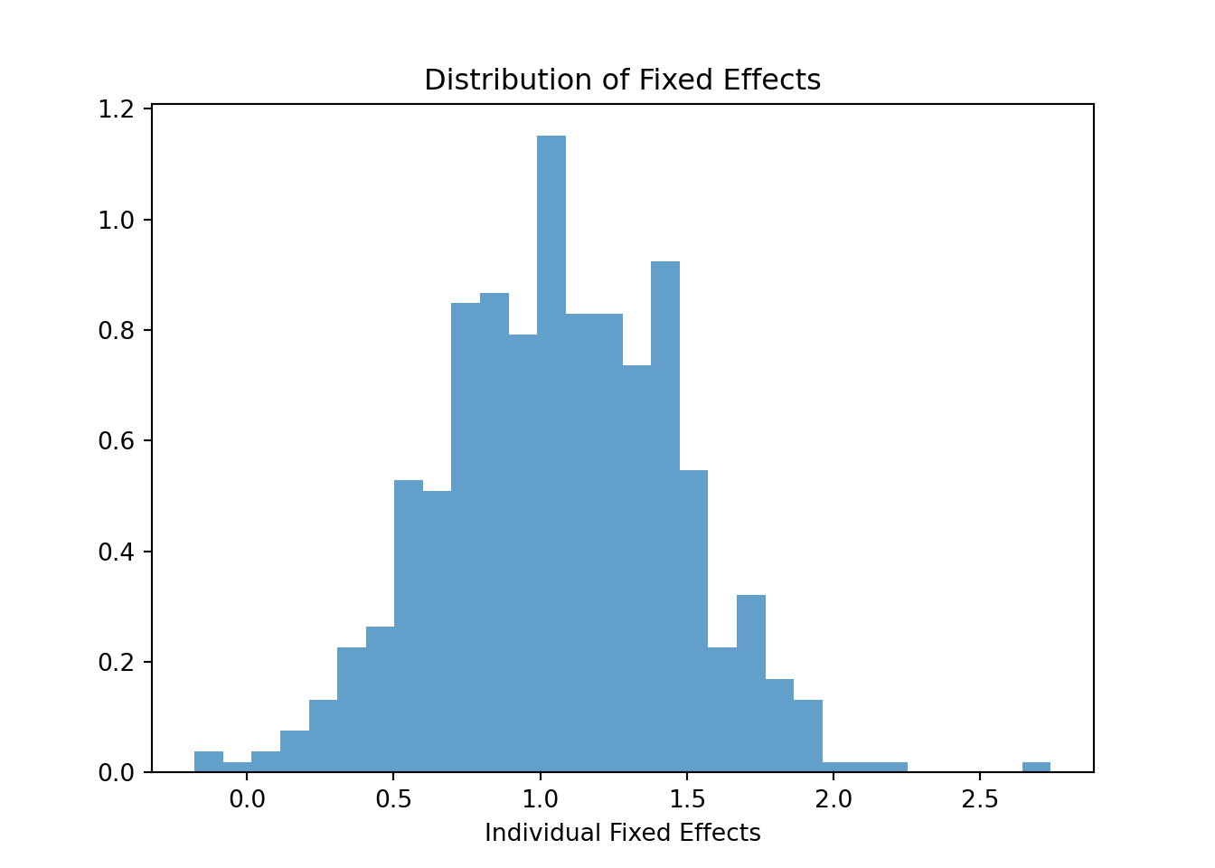
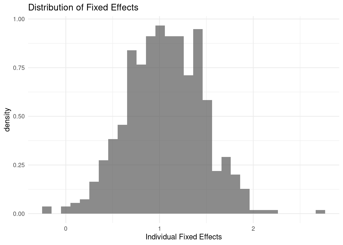
Visualizing Unobserved Heterogeneity
The “fixed effects” (\(\alpha_i\)) estimated in an FE model represent the time-invariant, unobserved characteristics of each individual (e.g., innate ability, motivation, family background) that affect their wage. Visualizing the distribution of these effects can reveal the extent of this heterogeneity.
Estimate a Fixed Effects model for lwage using exper, expersq, and union as predictors.
Extract the individual fixed effects from your estimated model.
Create a histogram or density plot to visualize the distribution of these fixed effects.
Interpret the plot: What does the shape and spread of the distribution tell you about the sample? Does it appear that unobserved, time-constant individual differences are an important factor in explaining wage variation?
The histogram shows a wide spread of fixed effects, suggesting substantial unobserved time-constant heterogeneity across individuals. Since these effects capture persistent individual differences not explained by the predictors, their significant variation implies that individual-specific factors play an important role in wage determination. The roughly bell-shaped but somewhat skewed distribution indicates most individuals cluster around the mean effect, with some outliers showing particularly high or low baseline wages.
Since \(\nu_{it}\) is defined as white noise, it is, by definition, not serially correlated. Therefore, the error term in the first-differenced model satisfies the classical OLS assumption of no serial correlation.
The FE error:
Let’s analyze the transformed error term, \(\tilde{\epsilon}_{it} = \epsilon_{it} - \bar{\epsilon}_i\), where \(\bar{\epsilon}_i = \frac{1}{T} \sum_{s=1}^{T} \epsilon_{is}\).
The de-meaned error at time \(t\) is: \(\tilde{\epsilon}_{it} = \epsilon_{it} - \frac{1}{T}(\epsilon_{i1} + \epsilon_{i2} + ... + \epsilon_{iT})\)
And the de-meaned error at time \(t-1\) is: \(\tilde{\epsilon}_{i,t-1} = \epsilon_{i,t-1} - \frac{1}{T}(\epsilon_{i1} + \epsilon_{i2} + ... + \epsilon_{iT})\)
To check for serial correlation, we need to determine if the covariance between \(\tilde{\epsilon}_{it}\) and \(\tilde{\epsilon}_{i,t-1}\) is zero.
Click to see why the covariance is nonzero explicitly.
To demonstrate mathematically that the covariance of the demeaned error term in a Fixed Effects (FE) model is nonzero when the original error term follows a random walk, we will expand the covariance expression and analyze its components.
The transformed error term in the FE model is \(\tilde{\epsilon}_{it} = \epsilon_{it} - \bar{\epsilon}_i\), where \(\bar{\epsilon}_i = \frac{1}{T} \sum_{s=1}^{T} \epsilon_{is}\). We want to show that \(Cov(\tilde{\epsilon}_{it}, \tilde{\epsilon}_{i,t-1}) \neq 0\).
Now, we need to calculate each of these components:
\(Cov(\epsilon_{it}, \epsilon_{i,t-1})\): As established from the properties of a random walk, for \(t > t-1\): \(Cov(\epsilon_{it}, \epsilon_{i,t-1}) = Var(\epsilon_{i,t-1}) = (t-1)\sigma_{\nu}^2\)
\(Cov(\epsilon_{it}, \bar{\epsilon}_i)\): \(Cov(\epsilon_{it}, \bar{\epsilon}_i) = Cov(\epsilon_{it}, \frac{1}{T}\sum_{s=1}^{T} \epsilon_{is}) = \frac{1}{T}\sum_{s=1}^{T} Cov(\epsilon_{it}, \epsilon_{is})\) This sum can be split into two parts: for \(s \le t\) and for \(s > t\).
For \(s \le t\), \(Cov(\epsilon_{it}, \epsilon_{is}) = Var(\epsilon_{is}) = s\sigma_{\nu}^2\).
For \(s > t\), \(Cov(\epsilon_{it}, \epsilon_{is}) = Var(\epsilon_{it}) = t\sigma_{\nu}^2\).
So, \(Cov(\epsilon_{it}, \bar{\epsilon}_i) = \frac{\sigma_{\nu}^2}{T} [\sum_{s=1}^{t} s + \sum_{s=t+1}^{T} t]\)\(= \frac{\sigma_{\nu}^2}{T} [\frac{t(t+1)}{2} + (T-t)t]\)
Combining these terms will result in a complex expression. However, we can see that each component is a function of \(t\) and \(T\), and they will not generally cancel each other out to zero. The demeaning process, by subtracting the individual-specific mean, introduces a common component (\(\bar{\epsilon}_i\)) into each transformed error term. Because the original error terms are strongly serially correlated in a random walk, this shared component does not eliminate the correlation. Instead, it creates a new, complex covariance structure.
Since the individual covariance terms are generally non-zero and do not cancel out, the overall \(Cov(\tilde{\epsilon}_{it}, \tilde{\epsilon}_{i,t-1})\) will be non-zero. This demonstrates that the error term in the FE transformed model remains serially correlated when the idiosyncratic error follows a random walk, making the FE estimator inefficient in this scenario.
Because \(\epsilon_{it}\) is a random walk, it is strongly serially correlated with its own past values. For instance, \(\epsilon_{it} = \epsilon_{i,t-1} + \nu_{it}\), and \(\epsilon_{i,t-1} = \epsilon_{i,t-2} + \nu_{i,t-1}\), and so on. This means that \(\epsilon_{it}\) is a sum of all past white noise shocks.
When we de-mean this series, the transformed error \(\tilde{\epsilon}_{it}\) becomes a complex combination of all the original error terms for that individual. Both \(\tilde{\epsilon}_{it}\) and \(\tilde{\epsilon}_{i,t-1}\) share the same subtracted mean, \(\bar{\epsilon}_i\), and their non-mean components, \(\epsilon_{it}\) and \(\epsilon_{i,t-1}\), are themselves highly correlated. The de-meaning process does not remove the underlying correlation structure of a random walk.
As a result, the covariance between the de-meaned errors, \(Cov(\tilde{\epsilon}_{it}, \tilde{\epsilon}_{i,t-1})\), will be non-zero. The transformed error term in the FE model remains serially correlated.
Step 2: Construct De-meaned Variables Using the formula \(\ddot{y}_{it} = y_{it} - \bar{y}_i\) and \(\ddot{x}_{it} = x_{it} - \bar{x}_i\):
Firm (i)
Year (t)
\(\ddot{y}_{it}\)
\(\ddot{x}_{it}\)
A
1
\(5 - 6 = -1\)
\(2 - 3 = -1\)
A
2
\(7 - 6 = 1\)
\(3 - 3 = 0\)
A
3
\(6 - 6 = 0\)
\(4 - 3 = 1\)
B
1
\(12 - 12 = 0\)
\(6 - 6 = 0\)
B
2
\(10 - 12 = -2\)
\(5 - 6 = -1\)
B
3
\(14 - 12 = 2\)
\(7 - 6 = 1\)
(b) The First Differences Estimator
Using the formulas \(\Delta y_{it} = y_{it} - y_{i,t-1}\) and \(\Delta x_{it} = x_{it} - x_{i,t-1}\). Note that the first observation for each firm (\(t=1\)) is lost.
Firm (i)
Year (t)
\(\Delta y_{it}\)
\(\Delta x_{it}\)
A
2
\(7 - 5 = 2\)
\(3 - 2 = 1\)
A
3
\(6 - 7 = -1\)
\(4 - 3 = 1\)
B
2
\(10 - 12 = -2\)
\(5 - 6 = -1\)
B
3
\(14 - 10 = 4\)
\(7 - 5 = 2\)
You are left with 4 observations in the differenced dataset. The general formula is \(N(T-1)\), where \(N\) is the number of individuals and \(T\) is the number of time periods. Here, \(2(3-1) = 4\).
Fixed Effects (FE) Model Errors
The error (residual) for the FE model is calculated using the de-meaned data with the formula: \(e_{it} = \ddot{y}_{it} - \beta \ddot{x}_{it}\)
Given \(\beta = 2\):
Firm (i)
Year (t)
\(\ddot{y}_{it}\)
\(\ddot{x}_{it}\)
Calculation of \(e_{it} = \ddot{y}_{it} - 2 \ddot{x}_{it}\)
FE Error (\(e_{it}\))
A
1
-1
-1
\(-1 - (2 \times -1)\)
1
A
2
1
0
\(1 - (2 \times 0)\)
1
A
3
0
1
\(0 - (2 \times 1)\)
-2
B
1
0
0
\(0 - (2 \times 0)\)
0
B
2
-2
-1
\(-2 - (2 \times -1)\)
0
B
3
2
1
\(2 - (2 \times 1)\)
0
First Differences (FD) Model Errors
The error (residual) for the FD model is calculated using the first-differenced data with the formula: \(\Delta e_{it} = \Delta y_{it} - \beta \Delta x_{it}\)
The Strict Exogeneity assumption states that the error term in any period \(t\) must be uncorrelated with the explanatory variables in all periods (past, present, and future) for a given individual \(i\). Formally, \(E(u_{it} | X_{i1}, ..., X_{iT}) = 0\).
The scenario describes a “feedback effect”: a past error term (\(u_{i,t-1}\)) influences a current explanatory variable (\(X_{it}\)). This means \(Cov(X_{it}, u_{i,t-1}) \neq 0\).
This violates strict exogeneity and causes bias in both estimators:
First Differences (FD): The FD model regresses \(\Delta X_{it}\) on \(\Delta u_{it}\). The covariance between the regressor and the new error term is: \(Cov(\Delta X_{it}, \Delta u_{it}) = Cov(X_{it} - X_{i,t-1}, u_{it} - u_{i,t-1})\) Expanding this covariance gives four terms, one of which is \(-Cov(X_{it}, u_{i,t-1})\). Since this term is non-zero by our scenario, the total covariance will be non-zero, and the FD estimator will be biased.
Fixed Effects (FE): The de-meaning process involves subtracting the mean \(\bar{x}_i\), which is a function of all \(X\)’s for that individual, including \(X_{it}\). Since \(X_{it}\) is correlated with \(u_{i,t-1}\), the de-meaned regressor \(\ddot{x}_{it}\) will also be correlated with the error term \(u_{i,t-1}\), violating the necessary conditions for consistency.
Choosing Between FE and FD
(a) Interpretation of Similar Results
The fact that the FE and FD estimators produce very similar results (0.15 and 0.18) is reassuring. Both methods are designed to control for unobserved time-invariant heterogeneity (\(\alpha_i\)). Their similarity suggests that the estimate of \(\beta\) is robust to the specific transformation method used. It provides confidence that the unobserved heterogeneity has been adequately addressed. It also gives suggestive (though not definitive) evidence that the strict exogeneity assumption holds, as a violation of this assumption could affect the two estimators differently and lead to divergent results.
(b) Correlation of -0.48
The choice between FE and FD depends on the time-series properties of the error term, \(u_{it}\). As shown in the lecture: * Theory: If the original errors \(u_{it}\) are serially uncorrelated (i.i.d.), then the first-differenced errors \(\Delta u_{it}\) will have a serial correlation of exactly -0.5.
A correlation of -0.48 is extremely close to -0.5. This is strong evidence that the underlying assumption of the FE model—that the idiosyncratic errors \(u_{it}\) are serially uncorrelated—is correct.
Conclusion: In this case, the Fixed Effects (FE) model is preferable. When its underlying assumptions hold, the FE estimator is more efficient (i.e., it has a smaller variance and produces smaller standard errors) than the FD estimator.
(c) Correlation of -0.05
A correlation of -0.05 is very close to zero and far from -0.5. This implies that the assumption of serially uncorrelated \(u_{it}\) is violated.
Theory: If the first-differenced errors \(\Delta u_{it}\) are serially uncorrelated (correlation near zero), it implies that the original error term \(u_{it}\) likely follows a random walk. A random walk process is defined as \(u_{it} = u_{i,t-1} + e_{it}\), where \(e_{it}\) is an i.i.d. shock. In this case, the first difference is \(\Delta u_{it} = e_{it}\), which is serially uncorrelated by definition.
Conclusion: In this scenario, the underlying assumptions of the FD model are met. The First Differences (FD) model is preferable because it is more efficient when the original errors follow a random walk.