Solutions Tutorial 6

Interpreting Binary Outcome Models

Compare the estimated coefficients on p401k across the three models. Do they agree on the direction and statistical significance of the effect of 401(k) eligibility on IRA participation?

Yes, all three models, LPM, Logit, and Probit, agree on the direction and statistical significance of the effect. In each model, the coefficient on p401k (401(k) Eligibility) is positive and statistically significant at the 1% level (p < 0.01). This indicates that being eligible for a 401(k) plan is associated with a higher probability of participating in an IRA.

Compare the estimated coefficients on inc across the three models. Do they agree on the direction and statistical significance of the effect of income on IRA participation?

Yes, the models also agree on the effect of income. The coefficient on inc (Income) is positive and statistically significant at the 1% level across all three models. This suggests that higher income is associated with a higher probability of participating in an IRA.

Interpret the coefficient on p401k from the LPM. What does this coefficient tell you about the effect of 401(k) eligibility on the probability of IRA participation?

The coefficient on p401k in the Linear Probability Model (LPM) is 0.057. Because the LPM models the probability directly, this coefficient can be interpreted as a marginal effect. It means that, on average, being eligible for a 401(k) plan is associated with a 5.7 percentage point increase in the probability of participating in an IRA, holding all other factors in the model constant. There is thus no crowding out, but rather crowding in of funds.

Are the R-squared values comparable across the three models? Why or why not?

No, the R-squared values are not directly comparable.

The LPM is estimated using Ordinary Least Squares (OLS), and its R-squared measures the proportion of the total variance in the binary outcome (pira) that is explained by the model.
The Logit and Probit models are estimated using Maximum Likelihood Estimation (MLE). The reported R-squared for these models is a “pseudo” R-squared (like McFadden’s R² or Cox-Snell R²). These metrics are derived from the log-likelihood function of the model and do not have the same “proportion of variance explained” interpretation as the OLS R-squared. They are useful for comparing nested models estimated with MLE but should not be directly compared to the OLS R-squared.

Model Estimation

First, we load the necessary libraries and data.

library(haven)
library(fixest)
library(modelsummary)
# Load Bertrand and Mullainathan (2004) data
lakisha <- read_dta('https://github.com/basm92/ee_website/raw/refs/heads/master/tutorials/datafiles/lakisha_aer.dta')

# Convert race to a factor for regression
lakisha$race <- factor(lakisha$race, levels = c('w', 'b'))

### a) Estimate a Linear Probability Model (LPM) regressing `call` on `race`.
lpm_race <- feols(call ~ race, data = lakisha, vcov = 'hc1')

### b) Estimate a Logit model with the same variables.
logit_race <- feglm(call ~ race, data = lakisha, family = 'logit', vcov = 'hc1')

### c) Estimate a Probit model with the same variables.
probit_race <- feglm(call ~ race, data = lakisha, family = 'probit', vcov = 'hc1')


modelsummary(list('LPM' = lpm_race,
                    'Logit'=logit_race,
                    'Probit' = probit_race), 
            stars = c('*' = .1, '**' = .05, '***' = .01),
            coef_map = c('raceb' = 'Black-Sounding Name'),
            gof_map = c('nobs', 'r.squared')
)

	LPM	Logit	Probit
* p < 0.1, p < 0.05, * p < 0.01
Black-Sounding Name	-0.032***	-0.438***	-0.217***
	(0.008)	(0.107)	(0.053)
Num.Obs.	4870	4870	4870
R2	0.003	0.006	0.006

import pandas as pd
import pyfixest as pf
import statsmodels.formula.api as smf
from statsmodels.iolib.summary2 import summary_col

df = pd.read_stata('https://github.com/basm92/ee_website/raw/refs/heads/master/tutorials/datafiles/lakisha_aer.dta')

# Convert race to a categorical variable
df['race'] = pd.Categorical(df['race'], categories=['w', 'b'], ordered=True)
 
## LPM
lpm = smf.ols('call ~ race', data=df).fit()
 
## Logit
logit = smf.logit('call ~ race', data=df).fit()

Optimization terminated successfully.
         Current function value: 0.278228
         Iterations 7

 
## Probit
probit = smf.probit('call ~ race', data=df).fit()

Optimization terminated successfully.
         Current function value: 0.278228
         Iterations 6

### Alternatives using pyfixest are:
# lpm = pf.feols('call ~ race', data = df)
# logit = pf.feglm('call ~ race', family='logit', data = df)
# probit = pf.feglm('call ~ race', family='probit', data = df)
# pf.etable([lpm, logit, probit])
 
# Display results in a table
print(summary_col([lpm, logit, probit],
            model_names=['LPM', 'Logit', 'Probit'],
            stars=True, info_dict={'N': lambda x: f"{int(x.nobs)}"}))


===============================================
                  LPM       Logit      Probit  
-----------------------------------------------
Intercept      0.0965***  -2.2366*** -1.3017***
               (0.0055)   (0.0686)   (0.0350)  
race[T.b]      -0.0320*** -0.4382*** -0.2165***
               (0.0078)   (0.1073)   (0.0528)  
R-squared      0.0035                          
R-squared Adj. 0.0033                          
N              4870       4870       4870      
===============================================
Standard errors in parentheses.
* p<.1, ** p<.05, ***p<.01

* Clear memory and set Stata to not pause for long output
clear all
set more off

* 1. Load the dataset from the URL
use "https://github.com/basm92/ee_website/raw/refs/heads/master/tutorials/datafiles/lakisha_aer.dta", clear

* 2. Estimate the Linear Probability Model (LPM)
* The `regress` command is Stata's OLS command.
tabulate(race),generate(r)
reg call r1, robust
estimates store lpm

* 3. Estimate the Logit model
logit call r1, robust
estimates store logit

* 4. Estimate the Probit model
probit call r1, robust
estimates store probit

* 5. Create a combined regression table
* The `esttab` command creates publication-quality tables.
* If you don't have it installed, run: ssc install estout
esttab lpm logit probit, star(* 0.1 ** 0.05 *** 0.01) b(%9.3f) se r2

All three models strongly agree that perceived race has a statistically significant effect on the probability of receiving a callback. The negative sign on the coefficient for a black-sounding name (raceb) indicates that these applicants have a lower probability of receiving a callback compared to applicants with white-sounding names.

Marginal Effects vs. Coefficients

Calculate the Average Marginal Effect (AME) of the race variable from your Logit and Probit models in the previous question.

library(marginaleffects)
avg_slopes(logit_race, variables='race')


 Estimate Std. Error     z Pr(>|z|)    S   2.5 %  97.5 %
   -0.032    0.00778 -4.11   <0.001 14.7 -0.0473 -0.0168

Term: race
Type: response
Comparison: b - w

avg_slopes(probit_race, variables='race')


 Estimate Std. Error     z Pr(>|z|)    S   2.5 %  97.5 %
   -0.032    0.00778 -4.11   <0.001 14.7 -0.0473 -0.0168

Term: race
Type: response
Comparison: b - w

from marginaleffects import *
avg_slopes(logit, variables='race')

shape: (1, 9)

term	contrast	estimate	std_error	statistic	p_value	s_value	conf_low	conf_high
str	str	f64	f64	f64	f64	f64	f64	f64
"race"	"b - w"	-0.032033	0.007783	-4.11555	0.000039	14.66008	-0.047288	-0.016778

avg_slopes(probit, variables='race')

shape: (1, 9)

term	contrast	estimate	std_error	statistic	p_value	s_value	conf_low	conf_high
str	str	f64	f64	f64	f64	f64	f64	f64
"race"	"b - w"	-0.032033	0.007783	-4.11555	0.000039	14.66008	-0.047288	-0.016778

* 6. Marginal effects for Logit
margins, dydx(race)

* 7. Marginal effects for Probit
margins, dydx(race)

Interpret the AME from the Probit model. What does this number tell you about the difference in callback probabilities between resumes with white-sounding and black-sounding names?

The Average Marginal Effect (AME) from the Probit model is -0.0320. This means that, on average, a resume with a black-sounding name has a 3.2 percentage point lower probability of receiving a callback compared to a resume with a white-sounding name.

How do the AMEs from the Logit and Probit models compare to each other? How do they compare to the coefficient on race from the LPM in Question 4? Discuss your findings.

Comparison: The AMEs from the Logit and Probit models are identical (-0.0320).
Comparison to LPM: These AMEs are also identical to the coefficient on raceb from the LPM (-0.0320).

Discussion: This result is expected and highlights a key feature of these models. When the model only contains a binary independent variable (like race), the non-linearities of the Logit and Probit models do not play a significant role in altering the average effect. The coefficient from the LPM directly estimates the average difference in probabilities between the two groups. The AMEs from the Logit and Probit models calculate this same average difference, so in this simple case, they yield the same numerical result. The underlying coefficients differ, but the implied effect on the probability is the same.

The Pros and Cons of Simplicity

What are the two main advantages of the LPM, particularly concerning estimation and interpretation?

Ease of Estimation: The LPM is estimated using OLS, a computationally simple and widely understood method.
Direct Interpretation: The coefficients of an LPM are directly interpretable as marginal effects. A coefficient \(\beta_k\) represents the change in the probability of the outcome for a one-unit change in the predictor \(x_k\), which is very intuitive.

What are its two primary shortcomings, as discussed in the lecture? Explain why each is a problem.

Predicted Probabilities Outside: The linear functional form can produce predicted values greater than 1 or less than 0. This is a logical impossibility, as probabilities must lie within the interval.
Inherent Heteroskedasticity: For a binary outcome, the variance of the error term depends on the values of the independent variables: \(Var(u|X) = p(X)(1-p(X))\), where \(p(X)\) is the probability of success. Since \(p(X)\) changes with \(X\), the variance is not constant. This violates the OLS assumption of homoskedasticity, making the standard errors and inference (t-tests, F-tests) invalid unless corrected.

One of these shortcomings can be partially addressed using robust standard errors. Which one is it, and why does this fix work?

Heteroskedasticity is the shortcoming addressed by using robust standard errors (e.g., Huber-White standard errors).

This fix works because robust standard errors are designed to be valid even when the model’s errors are not homoskedastic. They adjust the standard error calculation to account for the fact that the variance of the error term is not constant, thereby allowing for correct statistical inference (valid p-values and confidence intervals) even though the underlying model is misspecified in this way.

The Latent Variable Framework

In your own words, explain the concept of a latent variable \(y^*\) and how it relates to the observed binary outcome \(y\).

A latent variable, \(y^*\), is an unobserved, continuous variable that represents the underlying propensity or utility for an outcome to occur. We cannot measure it directly, but we can observe the choice or outcome, \(y\), that results from it. The relationship is that the binary outcome \(y\) equals 1 if the latent variable \(y^*\) crosses a certain threshold (typically normalized to zero), and \(y\) equals 0 otherwise.

For example, \(y^*\) could be the “net benefit” of having an IRA. If this net benefit is positive (\(y^* > 0\)), we observe the person getting an IRA (\(y=1\)). If it’s negative (\(y^* \le 0\)), we observe them not getting one (\(y=0\)).

The lecture states that \(P(y_i=1) = P(\epsilon_i > -X_i'\beta)\). What is the final step needed to get from this expression to the specific functional forms for the Probit and Logit models? What key assumption distinguishes the two models?

The final step is to assume a specific cumulative distribution function (CDF) for the error term, \(\epsilon_i\).

Since probability distributions are symmetric around zero, \(P(\epsilon_i > -X_i'\beta)\) is equivalent to \(P(\epsilon_i \le X_i'\beta)\). This is simply the CDF of \(\epsilon\) evaluated at \(X_i'\beta\).

The key assumption that distinguishes the two models is the choice of this distribution:

Probit Model: Assumes the error term \(\epsilon_i\) follows a standard normal distribution. Thus, \(P(y_i=1) = \Phi(X_i'\beta)\), where \(\Phi(\cdot)\) is the standard normal CDF.
Logit Model: Assumes the error term \(\epsilon_i\) follows a standard logistic distribution. Thus, \(P(y_i=1) = \Lambda(X_i'\beta)\), where \(\Lambda(\cdot)\) is the standard logistic CDF.

Understanding Maximum Likelihood

Explain the fundamental goal of MLE. How does its objective differ from the objective of OLS (which minimizes the sum of squared residuals)?

The fundamental goal of Maximum Likelihood Estimation (MLE) is to find the set of model parameters (\(\beta\)) that maximizes the probability of observing the actual data that were collected. It asks: “Given our observed data, what are the most likely parameter values that could have generated this data?”

This differs from OLS, whose objective is to minimize the sum of squared residuals (SSR). OLS finds the line (or hyperplane) that minimizes the vertical distance between the observed data points and the fitted line, without making any probabilistic assumptions about how the data were generated beyond the error term properties.

Using the “biased coin” example from the lecture (observing 7 heads in 10 flips), explain how you would construct the likelihood function. What value of p (the probability of heads) does MLE tell us is the best estimate, and why is this intuitive?

Let \(p\) be the unknown probability of getting heads. The outcome of each flip is a Bernoulli trial. The probability of observing a single head is \(p\), and the probability of observing a single tail is \((1-p)\).

Construct the Likelihood Function: The likelihood of the data is the joint probability of observing our specific sequence of 10 independent flips. For 7 heads (H) and 3 tails (T), this joint probability is the product of the individual probabilities: \(L(p | \text{data}) = P(\text{flip}_1) \times P(\text{flip}_2) \times \dots \times P(\text{flip}_{10})\) \(L(p | \text{data}) = p \times p \times p \times p \times p \times p \times p \times (1-p) \times (1-p) \times (1-p)\) The likelihood function is therefore: \[ L(p) = p^7 (1-p)^3 \]
MLE Estimate: MLE finds the value of \(p\) that maximizes this function. Through calculus (or simply intuition), this function is maximized when \(p = \frac{7}{10} = 0.7\).
Intuition: This result is highly intuitive. If you flip a coin 10 times and get 7 heads, your most reasonable guess for the underlying probability of getting a head is simply the proportion you observed in your sample, which is 70%. MLE formalizes this intuition.

The Complexity of Interaction Terms

Suppose you were to estimate a Probit model: \[ P(\text{call}=1 | X) = \Phi(\beta_0 + \beta_1 \text{race}_i + \beta_2 \text{female}_i + \beta_3 (\text{race}_i \times \text{female}_i)) \]

Explain why you cannot simply look at the sign and significance of \(\hat{\beta}_3\) to determine the sign and significance of the interaction effect on the probability of receiving a callback. How does this differ fundamentally from the interpretation of an interaction term in an LPM?

In a non-linear model like Probit, you cannot interpret \(\hat{\beta}_3\) directly as the interaction effect on the probability.

Reason: The marginal effect of any one variable on the probability depends on the values of all other variables in the model, because the effect is filtered through the non-linear CDF, \(\Phi(\cdot)\). The interaction effect on the probability is the change in the marginal effect of race for a change in female (or vice-versa). This is the cross-partial derivative: \[ \frac{\partial^2 P(\text{call}=1)}{\partial \text{race} \partial \text{female}} \] When you compute this derivative, the chain rule results in a complex expression that depends not only on \(\beta_3\) but also on \(\beta_1\), \(\beta_2\), and the levels of all variables inside \(\Phi(\cdot)\). Therefore, the sign and significance of the interaction effect on the probability can be different for different individuals in the data (e.g., it could be positive for one group and negative for another). The sign and significance of \(\hat{\beta}_3\) only tell you about the interaction effect on the latent variable, not the observed probability.

Difference from LPM: This is fundamentally different from an LPM. In an LPM, the model is linear: \[ P(\text{call}=1 | X) = \beta_0 + \beta_1 \text{race}_i + \beta_2 \text{female}_i + \beta_3 (\text{race}_i \times \text{female}_i) \] Here, the interaction term \(\beta_3\) has a direct and constant interpretation. It is the exact amount by which the effect of race on the probability of a callback changes if the applicant is female. The sign and significance of \(\hat{\beta}_3\) directly and fully describe the interaction effect.

Censoring and the Tobit Model

The researcher considers dropping the zero-expenditure observations and running an OLS regression on the remaining positive values. Why would this lead to biased estimates?

Dropping the zero-expenditure observations would lead to sample selection bias. The sample of people with positive spending is not random; it’s a group selected based on a criterion (spending > 0) that is correlated with the outcome being studied. The factors that determine whether someone spends anything on medication are likely related to the factors that determine how much they spend. By excluding the zeros, the OLS estimates would only describe the relationship for the sub-population of spenders, not the overall population, leading to biased and inconsistent estimates of the true effect.

The researcher then considers running OLS on the full sample, including the zeros. Why is this also problematic for estimating the relationship between income and medication spending?

Running OLS on the full sample is also problematic because it forces a single linear relationship onto two distinct processes: (1) the decision to spend any money at all, and (2) the decision of how much to spend, given that you are spending. The large cluster of observations at zero will pull the regression line downwards, likely attenuating (underestimating) the true effect of income on expenditure for those who do spend money. The assumptions of OLS (e.g., normally distributed errors) are also violated by the large mass of data at a single point (zero).

Explain why the Tobit model is designed to handle this specific type of data problem.

The Tobit model is designed for corner solution outcomes or censored data, which is exactly this situation. It correctly specifies that there is a latent (unobserved) continuous variable, say \(y^*\), representing the “desired” or “potential” level of spending. * If this desired spending \(y^*\) is positive, we observe the actual amount of spending. * If this desired spending \(y^*\) is zero or negative, we observe spending of zero (the corner solution).

By modeling this underlying latent variable, the Tobit model simultaneously accounts for both the probability of having a positive outcome (spending > 0) and the magnitude of that outcome when it is positive. This provides a more accurate estimate of the relationship between predictors like income and the propensity to spend on medication.

Estimating a Tobit Model

Load the Mroz dataset. Create a histogram or frequency table for the hours variable. Based on the distribution you observe, explain precisely why a Tobit model is a more appropriate choice than a standard OLS regression.

library(haven)
# Load Mroz (1976) data
mroz <- read_dta('https://github.com/basm92/ee_website/raw/refs/heads/master/tutorials/datafiles/MROZ.DTA')

# Create a histogram of hours
ggplot(mroz, aes(x = hours)) +
  geom_histogram(binwidth = 100, fill = "skyblue", color = "black") +
  labs(title = "Distribution of Hours Worked by Married Women (1975)",
       x = "Hours Worked",
       y = "Frequency") +
  theme_minimal()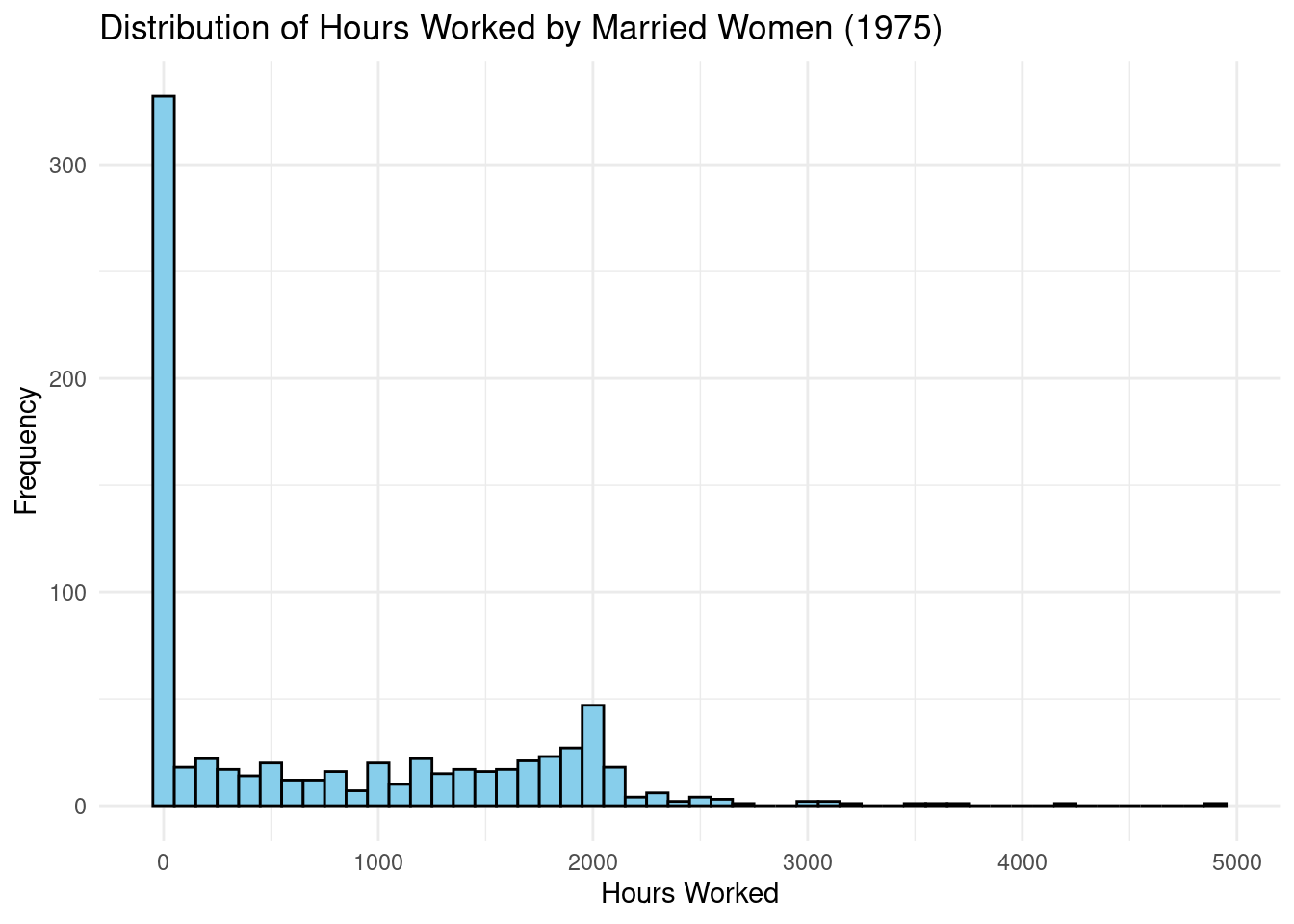

# Frequency of hours = 0
cat("Number of women with zero hours worked:", sum(mroz$hours == 0), "\n")

Number of women with zero hours worked: 325

cat("Percentage of women with zero hours worked:", round(100 * mean(mroz$hours == 0), 2), "%\n")

Percentage of women with zero hours worked: 43.16 %

import pandas as pd
import seaborn as sns
import matplotlib.pyplot as plt

mroz = pd.read_stata('https://github.com/basm92/ee_website/raw/refs/heads/master/tutorials/datafiles/MROZ.DTA')
# Set a visually appealing theme for the plots
sns.set_theme(style="whitegrid")

# Create a figure and axes for the plot
plt.figure(figsize=(10, 6))

# Create the histogram using seaborn
sns.histplot(data=mroz, x='hours', binwidth=100, color="skyblue", edgecolor="black")

# Set the title and labels using matplotlib
plt.title("Distribution of Hours Worked by Married Women (1975)", fontsize=16)
plt.xlabel("Hours Worked", fontsize=12)
plt.ylabel("Frequency", fontsize=12)

# Display the plot
plt.show()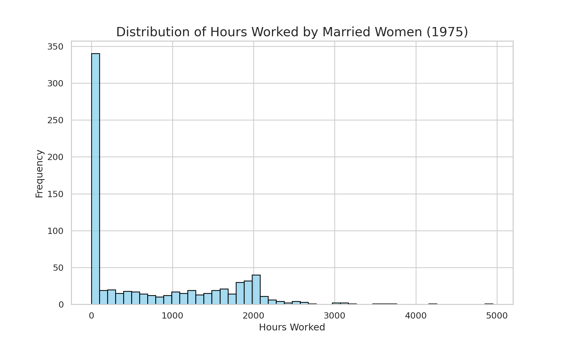

* 1. Load the Mroz dataset from Stata's web repository
* The 'clear' option ensures any data currently in memory is cleared first.
webuse mroz, clear

* 2. Generate the histogram with specified options
histogram hours, ///
    frequency ///
    width(100) ///
    fcolor(lightblue) ///
    lcolor(black) ///
    title("Distribution of Hours Worked by Married Women (1975)") ///
    xtitle("Hours Worked") ///
    ytitle("Frequency")

The histogram shows a large spike at hours = 0. Specifically, 325 out of the 753 women in the sample (43.16%) reported working zero hours. This is not a normally distributed variable; it is a censored distribution with a large mass of observations at the lower limit of zero.

A Tobit model is more appropriate than OLS because: 1. Censoring: The dependent variable is censored at zero. OLS would fail to account for the fact that a zero represents a “corner solution” and not just a low value on a continuous scale. 2. Two-Part Decision: Tobit correctly models the underlying process as a latent variable representing the “desire to work.” When this desire is below a certain threshold, observed hours are zero. This is a more realistic model of the labor supply decision than a simple linear model.

Estimate a Tobit model where hours is the dependent variable.

library(AER, quietly=TRUE)
# Estimate the Tobit model using the AER package
tobit_mroz <- tobit(hours ~ educ + exper + nwifeinc + kidslt6, data = mroz)

modelsummary(tobit_mroz, 
    stars = c('*' = .1, '**' = .05, '***' = .01),
    coef_map = c('educ' = 'Education (Years)', 
                 'exper' = 'Experience (Years)', 
                 'nwifeinc' = 'Non-wife Income (1000s)', 
                 'kidslt6' = 'Kids < 6',
                 '(Intercept)' = 'Constant'))

	(1)
* p < 0.1, p < 0.05, * p < 0.01
Education (Years)	113.229***
	(22.382)
Experience (Years)	58.045***
	(6.114)
Non-wife Income (1000s)	-15.945***
	(4.645)
Kids < 6	-610.422***
	(108.060)
Constant	-1233.300***
	(276.775)
Num.Obs.	753
AIC	7733.9
BIC	7761.7
RMSE	942.94

from py4etrics.tobit import Tobit # pip install py4etrics

# define a dummy for whether a value is 0
mroz['is_zero'] = (mroz['hours'] == 0).astype(int)

# the Tobit model from py4etrics needs an indication of which values are censored
# -1 indicates a censored value so we make the ones of our dummy is_zero negative
censor = - mroz['is_zero']

formula = 'hours ~ educ + exper + nwifeinc + kidslt6'
res_tobit = Tobit.from_formula(formula, cens=censor, left=0, data=mroz).fit()

Optimization terminated successfully.
         Current function value: 5.127429
         Iterations: 742
         Function evaluations: 1173

print(res_tobit.summary())

                              Tobit Regression Results                             
===================================================================================
Dep. Variable:                       hours   Pseudo R-squ:                    0.024
Method:                 Maximum Likelihood   Log-Likelihood:                -3861.0
No. Observations:                      753   LL-Null:                       -3954.9
No. Uncensored Obs:                    428   LL-Ratio:                        187.9
No. Left-censored Obs:                 325   LLR p-value:                     0.000
No. Right-censored Obs:                  0   AIC:                            7731.9
Df Residuals:                          748   BIC:                            7755.0
Df Model:                                4   Covariance Type:             nonrobust
==============================================================================
                 coef    std err          z      P>|z|      [0.025      0.975]
------------------------------------------------------------------------------
Intercept  -1233.2998    276.775     -4.456      0.000   -1775.768    -690.832
educ         113.2287     22.382      5.059      0.000      69.362     157.096
exper         58.0454      6.114      9.494      0.000      46.062      70.029
nwifeinc     -15.9452      4.645     -3.432      0.001     -25.050      -6.840
kidslt6     -610.4223    108.060     -5.649      0.000    -822.217    -398.628
Log(Sigma)     7.0831      0.037    189.670      0.000       7.010       7.156
==============================================================================

* 1. Install necessary user-written packages (if not already installed)
ssc install estout, replace

* 2. Load the Mroz dataset
webuse mroz

* 3. Estimate the Tobit model
* The 'tobit' command in Stata requires you to specify the lower limit (ll)
* Since hours worked is censored at 0, we use ll(0).
tobit hours educ exper nwifeinc kidslt6, ll(0)

* 4. Store the results for the table command
est store tobit_mroz

* 5. Generate the customized table using esttab

* Note on esttab options:
* starlevels(* 0.10 ** 0.05 *** 0.01): Customizes the significance star levels.
* label: Uses the variable labels instead of variable names (if set).
* titles(""): Removes the default model title.
* replace: Replaces an existing file (optional if outputting to a file).

esttab tobit_mroz, ///
    starlevels(* 0.10 ** 0.05 *** 0.01) ///
    nonotes nocons /// * Note: I've added 'nocons' to remove the constant, but you can keep it.
    label ///
    mtitles("Tobit Model (Hours Worked)") ///
    keep(educ exper nwifeinc kidslt6) ///
    rename(educ "Education (Years)" exper "Experience (Years)" nwifeinc "Non-wife Income (1000s)" kidslt6 "Kids < 6")

* If you want to include the constant:
* esttab tobit_mroz, starlevels(* 0.10 ** 0.05 *** 0.01) label mtitles("Tobit Model (Hours Worked)") rename(educ "Education (Years)" exper "Experience (Years)" nwifeinc "Non-wife Income (1000s)" kidslt6 "Kids < 6" _cons "Constant")

Focus on the estimated coefficient for kidslt6. Provide a careful interpretation of this coefficient.

The estimated coefficient for kidslt6 is -610.42.

Interpretation: This coefficient represents the marginal effect on the latent (unobserved) variable for hours worked, not on the observed hours themselves. The interpretation is: for each additional child under the age of 6, a woman’s underlying propensity or “desired” hours of work decreases by approximately 610 hours per year, holding education, experience, and other household income constant.

It is crucial to note that this is not the effect on expected hours worked for a woman who is already working. It is the effect on the underlying continuous variable that governs both the decision to work at all and how many hours to work if one does. The large, negative, and highly significant coefficient indicates that having young children is a very strong factor in reducing a married woman’s labor supply in this dataset.

Now estimate an OLS model. Compare your results with the Tobit model. Is this a valid comparison?

# Estimate the Tobit model using the AER package
ols_mroz <- lm(hours ~ educ + exper + nwifeinc + kidslt6, data = mroz)

modelsummary(ols_mroz, 
    stars = c('*' = .1, '**' = .05, '***' = .01),
    coef_map = c('educ' = 'Education (Years)', 
                 'exper' = 'Experience (Years)', 
                 'nwifeinc' = 'Non-wife Income (1000s)', 
                 'kidslt6' = 'Kids < 6',
                 '(Intercept)' = 'Constant'))

	(1)
* p < 0.1, p < 0.05, * p < 0.01
Education (Years)	48.424***
	(13.189)
Experience (Years)	37.632***
	(3.683)
Non-wife Income (1000s)	-7.005***
	(2.598)
Kids < 6	-273.788***
	(55.804)
Constant	-48.378
	(158.795)
Num.Obs.	753
R2	0.203
R2 Adj.	0.199
AIC	12172.9
BIC	12200.6
Log.Lik.	-6080.448
F	47.565
RMSE	777.45

import statsmodels.formula.api as smf
ols_mroz = smf.ols("hours ~ educ + exper + nwifeinc + kidslt6", data=mroz).fit()
summary_col([ols_mroz], stars=True,info_dict={'N': lambda x: f"{int(x.nobs)}"})

	hours
Intercept	-48.3784
	(158.7949)
educ	48.4237***
	(13.1894)
exper	37.6324***
	(3.6834)
nwifeinc	-7.0048***
	(2.5981)
kidslt6	-273.7879***
	(55.8038)
R-squared	0.2028
R-squared Adj.	0.1985
N	753

Standard errors in parentheses.
* p<.1, ** p<.05, ***p<.01

reg hours educ exper nwifeinc kidslt6

A direct comparison of the coefficients from the Tobit and OLS models is not valid. The OLS estimates are biased towards zero due to the model’s inability to correctly handle the censored nature of the hours variable. The OLS model incorrectly averages the zero and positive values of hours, which attenuates the estimated effects of the independent variables.

As expected, the absolute values of the coefficients in the OLS model are smaller than those in the Tobit model. This illustrates the downward bias of OLS in the presence of censoring. Because the underlying assumptions of OLS are violated, the resulting coefficients do not provide a consistent estimate of the relationships between the independent variables and the hours worked. Therefore, the Tobit model provides a more theoretically sound and econometrically appropriate analysis for this dataset.