| Event | Date | Subject |
|---|---|---|
| Lecture 1 | 21-04 | Introduction to Data and Data Science |
| Lecture 2 | 28-04 | Getting Data: API's and Databases |
| Lecture 3 | 07-05 | Getting Data: Web Scraping |
| Lecture 4 | 26-05 | Text as Data |
| Lecture 5 | 27-05 | Introduction to LLMs |
| Lecture 6 | 09-06 | Prompt Engineering and Structured Data |
| Lecture 7 | 16-06 | Spatial Data and Geocomputation |
Introduction to Applied Data Science
Lecture 1: Introduction to Data Science
Bas Machielsen
Introduction
Introduction
- This course aims to familiarize you with the basic aspects of data science and the process of data acquisition (APIs and Web Scraping)
- Independently collect and acquire data from online sources.
- Afterwards, we introduce students to the toolkit to process and analyze text data.
- Special attention is paid to LLM-related workflows.
- Finally, we will focus on the analysis of spatial data.
- Most of the applications and assignments in this course ask you to answer concrete economic questions.
- The philosophy behind these assignments is that you answer questions from the ground up, just like researchers do, and just like you will have to do at a later stage of your study.
- As such, this course is also an introduction into what economists do when they conduct empirical research.
- We develop these skills using the R programming language.
Overview
- Overview of the logistics (see course website for details.)
Learning Goals
- On effective completion of the course, students should:
- Understand the basics of R programming in a data science context
- Be able to independently acquire data from a variety of sources
- Understand and be able to analyze non-standard formats of data such as text and spatial data
- Be able to integrate code in reporting, thereby writing reproducible code and analysis
Who am I?
- Bas Machielsen (a.h.machielsen@uu.nl)
- Assistant Professor in Applied Economics at UU
- Teach various classes:
- Introduction to Applied Data Science (BSc 1st year)
- Applied Economics Research Course (BSc 3rd year)
- Empirical Economics (MSc)
- Research: Economic history & Political economy
- Lots of unstructured data (historical documents)
- And lots of econometric challenges
- Use machine learning and AI on a daily basis to solve these problems
Course Structure
- Course Website
- Course format: 7 Lectures and 8 Tutorials
- In 7 of the tutorials, we’ll focus on an in-depth explanation of the content of the lecture
- One will be dedicated to discussion of the mid-term exam
- The course will have a mid-term exam (40% of grade) and a final exam (60% of grade)
- \(4.5 \leq \text{Grade} \leq 5.5 \rightarrow\) Retake (counts for 100%).
- These exams will be conducted in person using pen and paper.
- Mock exams will be available on the course website.
- Pen and paper because the university does not support “nicer” ways of testing (sorry).
Introduction to Data and Data Science
Theoretical vs. Empirical Research
- Two kinds of research: theoretical and empirical
- Think of theoretical research as working with ideas and logic, while empirical research is about working with real-world data.
- Empirical research tests ideas against actual observations and data. You collect evidence from the real world—through experiments, surveys, datasets, or observations—and use statistical methods to analyze patterns and relationships.
- Within empirical research, three objectives:
- To measure a quantity of interest, such as a country’s Gross Domestic Product (GDP).
- To predict a quantity of interest, such as stock prices.
- To explain a quantity of interest, such as the effect of education on earnings.
Prediction
- The primary goal of prediction is to forecast the value of a dependent variable (\(Y\)) as accurately as possible based on a set of independent variables (\(X\)).
- Our focus is on \(\hat{y}\): This is the predicted value of \(Y\) generated by our model.
- We build a model that minimizes the difference between the actual values (\(Y\)) and the predicted values (\(\hat{y}\)). This difference is known as the residual.
- We are less concerned with the individual coefficients of the independent variables, as long as the model as a whole produces accurate forecasts.
Example: Prediction
Predicting next quarter’s GDP growth using indicators like inflation, consumer confidence, and employment data. The main goal is the accuracy of the GDP forecast (\(\hat{y}\)), not necessarily the isolated impact of each indicator.
Explanation
- The goal of causal inference is to determine the specific impact of one variable on another, holding all other relevant factors constant.
- Our focus is on \(\hat{\beta}\): This is the estimated coefficient of an independent variable. It quantifies the direction and magnitude of the relationship between an independent variable and the dependent variable.
- We aim to obtain an unbiased estimate of the true underlying relationship (\(\beta\)). The “hat” on \(\beta\) means that it is an estimate derived from our sample data.
- What matters most is whether our coefficient \(\hat{\beta}\) is a “good approximation” of the true \(\beta\). We are deeply concerned about issues like omitted variable bias, as they can lead to incorrect conclusions about the causal effect of a variable.
Empirical Research
Example: Empirical Research in Economics
A recent example of empirical research from a top economics journal is “When Do Nudges Increase Welfare?” by Hunt Allcott, Daniel Cohen, William Morrison, and Dmitry Taubinsky, published in the American Economic Review
This study examines whether “nudges”—small interventions designed to influence behavior, like nutrition labels on soda—actually improve social welfare. The researchers used real-world data on consumer behavior to test theoretical assumptions about how these policies work.
They analyzed how different consumers respond to interventions like nutritional labels on sugary drinks.
The research revealed that nudges may influence the “wrong people” – for instance, moderate soda drinkers who already consume responsibly might reduce consumption after seeing labels, while heavy consumers (the intended target) might ignore them entirely.
Why Data Science?
- Contemporary economics does a lot of empirical work.
- The data used in economics research comes from a wide variety of sources, and the analyses are getting more and more diverse.
Example: Diverse Data
Ashraf and Galor (2013) argue that genetic diversity has had a hump-shaped effect on economic development—populations with intermediate diversity (like Europeans and Asians) developed more successfully than those with very high diversity (Africans) or very low diversity (Native Americans).
For genetic diversity data, they primarily used the HGDP-CEPH Human Genome Diversity Cell Line Panel, which provided data from 53 ethnic groups across 21 countries, measuring expected heterozygosity (the probability that two randomly selected individuals differ genetically).
For economic outcomes, they used historical population density estimates from McEvedy and Jones (1978) for the years 1 CE, 1000 CE, and 1500 CE, and income per capita data for 2000 CE.
Why Data Science? [2]
- Economics has dramatically expanded its conception of what counts as data.
- While traditional economics focused on estimating causal parameters using structured datasets, Mullainathan argues that prediction problems require different tools, opening economics to face recognition data, text analysis, and real-time behavioral traces.
- This shift means that as data scientists, you’ll need skills beyond regression analysis:
- From handling unstructured text and images to understanding how algorithms can both reveal and perpetuate social inequalities in ways traditional economic data never captured.
Example: Diverse Data
Sendhil Mullainathan’s work with machine learning has shown economists how to extract insights from unconventional sources—from medical records revealing patterns in doctor decision-making to satellite imagery predicting poverty .
Introduction to Data
What exactly are data?
- Think of data as organized information that helps us answer questions. The simplest way to picture data is a spreadsheet—like an Excel file with rows and columns.
- Each row represents an observation or unit we’re studying. For example, if you’re studying students, each row might be one student. If you’re studying countries, each row is one country.
- Each column represents a variable or characteristic we’ve measured. For the student example, columns might include: name, age, major, GPA, hours studied per week, coffee consumption, or hometown.
- Where a row and column meet is a data point—a specific piece of information. So if we look at row 5 (student Maria) and column 3 (major), we might find “Economics.”
Example: Data
- Example of a simple data set:
# A tibble: 5 × 8
  student_id name     age major          gpa hours_studied has_job hometown
       <int> <chr>  <dbl> <chr>        <dbl>         <dbl> <lgl>   <chr>
1          1 Maria     19 Economics      3.7            15 TRUE    Amsterdam
2          2 Ahmed     20 Data Science   3.9            20 FALSE   Cairo
3          3 Sophie    18 Economics      3.5            12 TRUE    Paris
4          4 James     19 Business       3.2            10 TRUE    London
5          5 Yuki      21 Data Science   3.8            18 FALSE   Tokyo
Example: Data
- This is a simple example dataset in R.
- In R (and in this class), we call this a data frame: R’s version of a spreadsheet.
- Data contains 5 students and various characteristics about them.
- Each row represents one student, and each column captures a different variable: their ID number, name, age, major, GPA, weekly study hours, whether they have a part-time job, and their hometown.
- Notice how we have different types of data:
- Numeric: age, gpa, hours_studied
- Character/text: name, major, hometown
- Logical/boolean: has_job (TRUE or FALSE)
Tidy Data
- Not all data is equally easy to work with. Some are messy and hard to work with, while others are “tidy” and make analysis smooth.
- Tidy data follows three simple principles:
- Each variable gets its own column
- Every characteristic you’re measuring should be in exactly one column. Don’t mix different types of information in the same column. For example, don’t have a column called “grades” that contains “Math: 8.5, English: 7.2”—split these into separate columns for math_grade and english_grade.
- Each observation gets its own row
- Every unit you’re studying (person, country, company) should occupy exactly one row. If you’re studying students and you measure them over time, each student-time combination gets its own row. Don’t put “Student 1’s grades in year 1, year 2, year 3” all in one row with columns like “grade_year1, grade_year2, grade_year3.”
- Each value gets its own cell
- A single cell should contain only one piece of information. Don’t cram multiple values into one cell, like “Amsterdam, Netherlands” in a single cell—split it into city and country columns.
Why does this matter?
- When data are tidy, you can quickly filter, summarize, and visualize without wrestling with the format.
- Most statistical software (like R’s tidyverse) is designed to work seamlessly with tidy data.
- Messy data forces you to spend hours cleaning before you can even start analyzing—and in real projects, data cleaning often takes 80% of your time.
- Learning to recognize and create tidy data from the start will save you countless headaches throughout your career in data science and economics.
- There are lots of datasets that do not naturally fit in this paradigm, including images, sounds, trees, and text.
- But rectangular data frames are extremely common in science and industry, and they are a great place to start your data science journey.
Example: Tidy Data
# A tibble: 10 × 8
   species island    bill_length_mm bill_depth_mm flipper_length_mm body_mass_g
   <fct>   <fct>              <dbl>         <dbl>             <int>       <int>
 1 Adelie  Torgersen           39.1          18.7               181        3750
 2 Adelie  Torgersen           39.5          17.4               186        3800
 3 Adelie  Torgersen           40.3          18                 195        3250
 4 Adelie  Torgersen           NA            NA                  NA          NA
 5 Adelie  Torgersen           36.7          19.3               193        3450
 6 Adelie  Torgersen           39.3          20.6               190        3650
 7 Adelie  Torgersen           38.9          17.8               181        3625
 8 Adelie  Torgersen           39.2          19.6               195        4675
 9 Adelie  Torgersen           34.1          18.1               193        3475
10 Adelie  Torgersen           42            20.2               190        4250
# ℹ 2 more variables: sex <fct>, year <int>
Example: Untidy Data
# A tibble: 10 × 5
   species island       id var               value
   <chr>   <chr>     <int> <chr>             <chr>
 1 Adelie  Torgersen     1 bill_length_mm    39.1
 2 Adelie  Torgersen     1 bill_depth_mm     18.7
 3 Adelie  Torgersen     1 flipper_length_mm 181
 4 Adelie  Torgersen     1 body_mass_g       3750
 5 Adelie  Torgersen     1 sex               male
 6 Adelie  Torgersen     1 year              2007
 7 Adelie  Torgersen     2 bill_length_mm    39.5
 8 Adelie  Torgersen     2 bill_depth_mm     17.4
 9 Adelie  Torgersen     2 flipper_length_mm 186
10 Adelie  Torgersen     2 body_mass_g       3800
Example: Untidy Data
# A tibble: 5 × 7
  Cursus        ECB1ID                             ...3  ...4  ...5  ...6  ...7
  <chr>         <chr>                              <chr> <chr> <chr> <chr> <chr>
1 Naam          Introduction to Applied Data Scie… <NA>  Resu… USE   <NA>  <NA>
2 Collegejaar   2024                               <NA>  <NA>  <NA>  <NA>  <NA>
3 <NA>          <NA>                               <NA>  <NA>  <NA>  <NA>  <NA>
4 <NA>          Deadline handing in grades: withi… <NA>  <NA>  <NA>  <NA>  <NA>
5 Studentnummer Naam                               Midt… Endt… Fina… Reta… Fina…
Introduction to R
Why R?
- From R for Data Science:
We think R is a great place to start your data science journey because it is an environment designed from the ground up to support data science. R is not just a programming language, but it is also an interactive environment for doing data science. To support interaction, R is a much more flexible language than many of its peers. This flexibility comes with its downsides, but the big upside is how easy it is to evolve tailored grammars for specific parts of the data science process. These mini languages help you think about problems as a data scientist, while supporting fluent interaction between your brain and the computer.
Why R?
- R is one of the most important data science languages (next to Python).
- It’s free, open-source, and used by data scientists, economists, and researchers worldwide.
- R is quite easy to learn and user friendly.
- Even though you might not agree when you are frustrated.
- It has great and transparent documentation.
- Think of it as a powerful calculator that can handle entire datasets, create visualizations, and run complex analyses—all through written commands instead of clicking buttons.
- In this class, the focus is on understanding the code and its output.
- You don’t have to write (much) code yourself.
What are objects?
- Objects are containers that store information in R.
- When you create that student dataset I showed earlier, we stored it in an object called
student_data. - Think of objects like labeled boxes: you put something in the box, give it a name, and can retrieve it later. You create objects using the assignment operator
<-:
- Now
my_ageholds the number 19,my_nameholds the text “Maria”, and my_grades holds a vector (list) of three numbers. Once created, you can use these objects in calculations:my_age + 1gives you 20.
What are functions?
- Functions are pre-written recipes that perform specific tasks.
- They take inputs (called arguments), do something with them, and return outputs.
- You recognize functions by their parentheses:
function_name(). For example:
Why do we need functions?
- Functions save you from reinventing the wheel.
- Instead of writing code to calculate an average yourself, you just use
mean(). - R comes with hundreds of built-in functions, and you can load packages (collections of related functions) for specialized tasks.
- You can even write your own functions when you need to repeat the same operation multiple times.
- The beauty of R is combining objects and functions: you store data in objects, then apply functions to analyze that data efficiently.
Packages
- A package (also called a library) is a collection of functions, datasets, and tools that someone has bundled together to solve specific problems.
- R comes with essential functions like
mean()andsum()but packages extend R’s capabilities enormously—like adding apps to your phone. - Imagine you want to create beautiful visualizations, scrape data from websites, or run machine learning algorithms.
- You could write all that code from scratch, but that would take months or years.
- Instead, experts have already written, tested, and shared packages that do this work for you.
Working with R
Downloading and installing R
- R is completely free, and installing it is straightforward. Here’s how to do it for your operating system:
- Go to https://cran.r-project.org/
- Click on “Download R for Linux”
- Choose your distribution (Ubuntu, Debian, Fedora, etc.)
- Follow the specific instructions for your distribution—this usually involves adding a repository and using your package manager
- For Ubuntu/Debian, you’ll typically open Terminal and run commands like:
- R is now installed! Type
Rin the terminal to start it
- Go to https://cran.r-project.org/
- Click on “Download R for macOS”
- Look for the first .pkg file under “Latest release” (make sure it matches your Mac’s processor—M1/M2/M3 Macs need the “arm64” version, older Intel Macs need the other version)
- Download and open the .pkg file
- Follow the installation prompts (you may need to enter your Mac password)
- R is now installed! You can find it in your Applications folder
- Go to https://cran.r-project.org/
- Click on “Download R for Windows”
- Click on “base” (this is the basic R installation)
- Click on the large download link at the top (something like “Download R-4.4.2 for Windows”)
- Once downloaded, double-click the .exe file and follow the installation wizard
- Just click “Next” through all the default options—they’re fine for beginners
- R is now installed! You’ll find it in your Start menu
IDE
- To work with R, we usually make use of an integrated development environment (IDE).
- Think of R as the engine and the IDE as the comfortable car built around it—you could drive the engine alone, but it’s much nicer with a proper interface!
- The IDE as your complete workspace for coding—it’s where you write your code, run it, see your results, view your data, and create visualizations, all in one place.
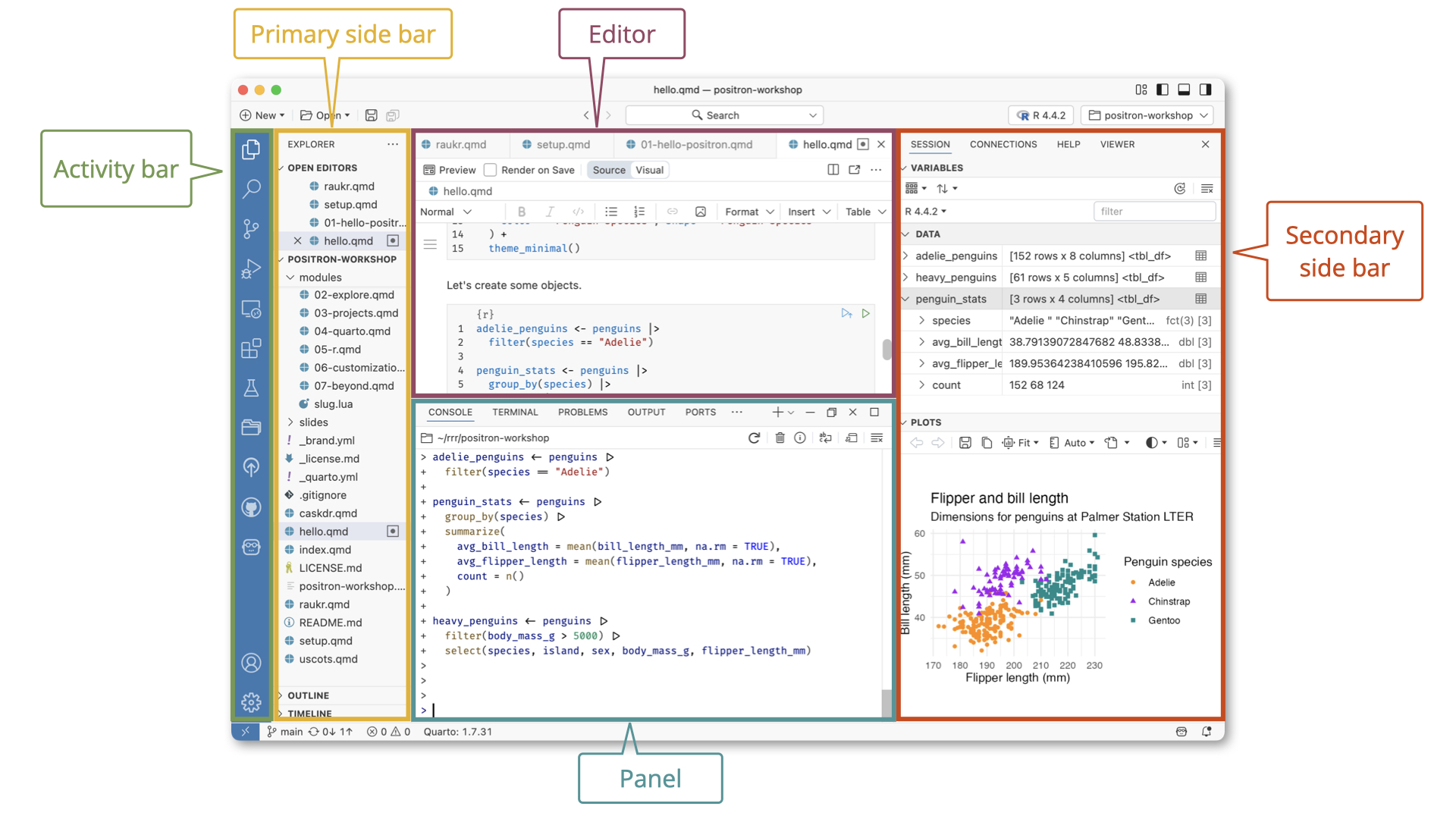
- Positron is a brand-new integrated development environment (IDE) created by Posit that’s designed specifically for data science work in both R and Python.
- Alternative choices: RStudio, VSCode (in other courses, but not necessary).
Positron
- Download and install Positron (here)
- Positron is a new IDE (the successor of RStudio) that “(..) unifies exploration and production work in one free, AI-assisted environment, empowering the full spectrum of data science in Python and R.”
- In other words, it’s going to be good at both Python and R
- Ability to smoothly work with both useful in whatever you’re going to do.
Positron Introduction
Organizing a Project
Positron and Projects
From the Positron Website:
Expert data scientists keep all the files associated with a given project together — input data, scripts, analytical results, and figures. This is such a wise and common practice, in data science and in software development more broadly, that most integrated development environments (IDEs) have built-in support for this practice.
- A Positron (or VS Code) workspace is often just a project folder that’s been opened in its own window via Open Folder or similar.
Workspaces
- When you work with R, you need to understand where your files live and where R is “looking” for them. This is called your workspace or working directory.
- A workspace is simply a folder on your computer where you keep all the files related to a specific project. For example, you might create a folder called
intro_adsthat contains:- Your R script files (.R)
- Your datasets (.csv, .xlsx)
- Your output (graphs, tables)
- Your written report
What is a working directory?
- The working directory is the folder that R is currently “paying attention to.”
- When R runs, it’s always positioned in some folder on your computer—that’s your working directory.
- You can check where R thinks it is by typing:
- This might return something like:
/Users/bas/Documents/intro_ads
Why does this matter?
- When you tell R to read a file, it looks in the working directory first.
- If your working directory is set to your project folder, you can simply write:
- R will look for “students.csv” in that folder.
- If your working directory is somewhere else (like your Desktop), R won’t find the file and will give you an error: “cannot open file ‘students.csv’: No such file or directory.”
Working directories
- In general, computers organize files and directories like trees.
- Your computer organizes files in nested folders, like branches on a tree. For example:
C:/Users/Bas/Documents/my_project/data.csv- Think of it as: Computer → Users → Bas → Documents → my_project → data.csv
Example file tree
- From a particular working directory, you can move to folders up the tree by means of
../, and down the tree with a folder’s name.
- Suppose this is your file tree:
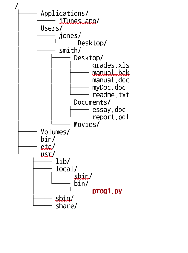
- E.g. if your working directory is
~/Users/jones/Desktop/, you can move to applications by../../../Applications - Or if your working directory is
~/bin, you can move tolocalby../usr/local.
Three ways to tell R where files are
- Three ways to tell R where files are:
- Full path from the root:
C:/Users/Bas/Documents/my_project/data.csv(Windows) or/Users/Maria/Documents/my_project/data.csv(Mac/Linux) - From your home directory using
~:~/Documents/my_project/data.csv. The~symbol is shorthand for “my home folder” (usuallyC:/Users/yournameon Windows or/Users/yournameon Mac) - From your current working directory using
.:./data.csvmeans “look in my current folder”
- Full path from the root:
- Use
../to go up one level: if you’re in my_project, then ../other_project/moves up to Documents, then intoother_project
The list.files() function
- In Positron, use
list.files()to see what’s in different locations:list.files(".")shows files in your current working directorylist.files("~")shows files in your home directorylist.files("./data")shows files in the “data” subfolder
- Best practice: Create one folder per project, set it as your working directory, and keep all your files there.
- This keeps everything organized and your file paths simple!
Console vs. Script
- When you open a project in Positron (or RStudio), the console’s working directory is automatically set to your project folder.
- If your project is in
~/Documents/my_project/, then when you type commands directly into the console:
- If your project is in
- However, when you launch a script (.R) or an Quarto (.qmd) document (we’ll see what it is later), its working directory is the folder where the .qmd file itself lives, not the project root!
- This causes a common frustration: your code works in the console but breaks when you launch a script.
- The fix is to use the
herelibrary, which always references the project root. - Let’s now proceed installing libraries.
- The fix is to use the
Installing libraries
Libraries
- Before proceeding to do anything else, it is useful to download and install a couple of libraries.
- Libraries can be installed with the
install.packages()functions. - Do not put this line of code in your scripts.
- Installing a package means downloading it from the internet and storing it on your computer’s hard drive. Just like downloading Netflix or Spotify onto your phone, you only need to do this once per computer.
- You should install packages in the console, not in your R script.
- The first libraries we should install are the
hereandtidyverselibraries.
Loading libraries
- Loading a package means telling R: “Hey, I want to use the functions from this package right now.”
- Even though the package is installed on your computer, R doesn’t automatically load all your packages when it starts up—that would be slow and waste memory.
The here library
- The
herelibrary always makes the path start from the project root (i.e. the folder in which you store all your files and which you opened in Positron).
The Rtools library
- If you’re using Windows,
Rtoolsallows you to install other packages faster and more efficiently. - To install
Rtools, use theinstall.packages()function and load it with:
Quarto
Quarto
- Quarto is a tool that lets you combine text, code, and output (like graphs and tables) into a single document.
- Think of it as a supercharged Word document where you can write your analysis, run R code, and see the results all in one place—and then export it as a PDF, HTML webpage, or Word document.
- Why use Quarto instead of just Word? In Word, you’d:
- Run analysis in R
- Copy a graph and paste it into Word
- Copy some results and type them into Word
- Realize you made a mistake in your data
- Re-run everything and copy-paste again (ugh!)
- With Quarto, you write your analysis and explanations together.
- When you click “Render,” Quarto automatically runs your R code, generates the graphs and tables, and creates a beautiful formatted document.
Quarto and R
- Quarto is language-agnostic (it works with R, Python, and other languages), but it’s perfect for R users.
- You write your R code in special “code chunks” within your document, and Quarto runs that code and includes the results.
- In Positron, click “New” in the top menu bar.
- Select “New File”
- Choose Quarto Document (you’ll see it has a .qmd extension)
- A new document will appear.
Understanding Quarto documents
- Your new .qmd file will have three parts:
- YAML Header (at the top, between — marks):
---
title: "My First Analysis"
author: "Your Name"
format: html
---- This controls document settings like title, author, and output format.
Understanding Quarto documents [2]
- Regular Text (markdown): Just type normally! You can add formatting:
**bold**for bold*italic*for italic# Headingfor headings## Subheadingfor subheadings
Understanding Quarto documents [3]
- Code Chunks:
Example Quarto document
- Copy and paste the example document below into an empty quarto document and click “Preview”.
---
title: "Student Analysis"
author: "Bas"
format: html
---

## Introduction

This is my analysis of student data.

```{r}
# Load libraries
library(tidyverse)

# Create data
students <- data.frame(
  name = c("Alice", "Bob", "Charlie"),
  grade = c(8.5, 7.2, 9.0)
)

# Show the data
print(students)

# Calculate average
mean(students$grade)
```

## Results

The average grade is shown above!
Recapitulation
Recapitulation
- We’ve seen the various objectives of data science.
- We have been introduced to the R language.
- We have seen that R consists of objects and functions.
- We have seen Positron, an integrated development environment (IDE) for R.
- We have seen the Quarto publication system, integrating R and text.
- In the first tutorial: Quarto documents and Data structures in R.
![]()
Lecture 1: Introduction to Data Science