| Event | Date | Subject |
|---|---|---|
| Lecture 1 | 21-04 | Introduction to Data and Data Science |
| Lecture 2 | 28-04 | Getting Data: API's and Databases |
| Lecture 3 | 07-05 | Getting Data: Web Scraping |
| Lecture 4 | 26-05 | Text as Data |
| Lecture 5 | 27-05 | Introduction to LLMs |
| Lecture 6 | 09-06 | Prompt Engineering and Structured Data |
| Lecture 7 | 16-06 | Spatial Data and Geocomputation |
Introduction to Applied Data Science
Lecture 7: Spatial Data
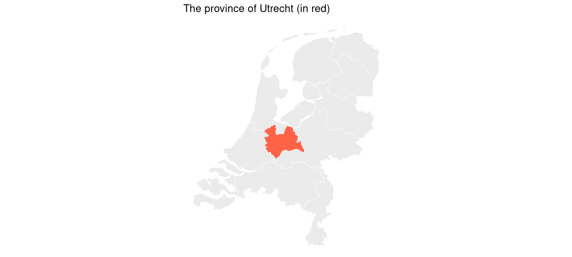
Our Running Example: The Province of Utrecht
- We will spend most of this lecture in one place: the Netherlands, and especially the province of Utrecht.
- We will answer increasingly interesting “where” questions about towns, stations, and shops.
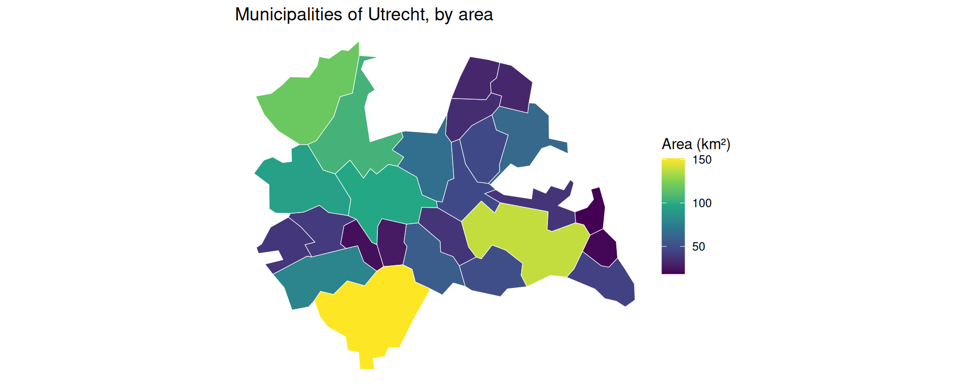
Loading Data: Municipalities of Utrecht
- Let’s get the municipalities (gemeenten) of the Netherlands from Statistics Netherlands using the
cbsodataRpackage you met in the API lecture. - We then keep only the municipalities of the province of Utrecht.
library(sf); library(dplyr); library(ggplot2); library(cbsodataR)

# The municipalities of the province of Utrecht (2022)
utrecht_names <- c(
  "Amersfoort","Baarn","De Bilt","Bunnik","Bunschoten","Eemnes",
  "Houten","De Ronde Venen","Lopik","Montfoort","Nieuwegein",
  "Oudewater","Renswoude","Rhenen","Soest","Stichtse Vecht",
  "Utrecht","Utrechtse Heuvelrug","Veenendaal","Vijfheerenlanden",
  "Wijk bij Duurstede","Woerden","Woudenberg","IJsselstein","Zeist")

# All Dutch municipalities as polygons, then keep the province of Utrecht
gemeenten <- cbs_get_sf("gemeente", 2022)
utrecht <- gemeenten |> filter(statnaam %in% utrecht_names)

ggplot(utrecht) + geom_sf(fill = "grey90", colour = "white") + theme_void()
Making Maps with geom_sf()
- A map is just a
ggplot. We usegeom_sf()and map an attribute to thefillcolour.
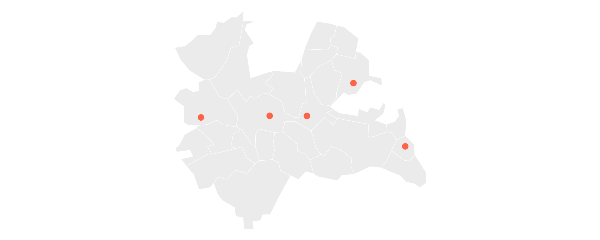
Example: Joining Points to Municipalities
Example: Spatial Join
First, build a small, fully reproducible set of well-known places as an sf object with st_as_sf(). Note the ritual: we set the points to EPSG:4326, then transform them to match utrecht.
places <- tibble::tribble(
  ~name,          ~lon,   ~lat,
  "Utrecht CS",   5.110,  52.089,
  "Amersfoort",   5.387,  52.156,
  "Zeist",        5.233,  52.089,
  "Veenendaal",   5.558,  52.027,
  "Woerden",      4.883,  52.085
) |>
  st_as_sf(coords = c("lon", "lat"), crs = 4326) |>
  st_transform(st_crs(utrecht))   # match the municipalities' CRS!

places
Simple feature collection with 5 features and 1 field
Geometry type: POINT
Dimension: XY
Bounding box: xmin: 120441.2 ymin: 448753.5 xmax: 166721.9 ymax: 463092.1
Projected CRS: Amersfoort / RD New
# A tibble: 5 × 2
name geometry
* <chr> <POINT [m]>
1 Utrecht CS (136001.7 455673.9)
2 Amersfoort (154986.1 463092.1)
3 Zeist (144431.6 455648.9)
4 Veenendaal (166721.9 448753.5)
5 Woerden (120441.2 455312.6)We can plot the points on top of the municipalities:
st_join() works like left_join(), but it matches a point to the polygon that contains it:
# A tibble: 5 × 2
  name       statnaam
* <chr>      <chr>
1 Utrecht CS Utrecht
2 Amersfoort Amersfoort
3 Zeist      Zeist
4 Veenendaal Veenendaal
5 Woerden    Woerden
Each point now carries the name of the municipality it sits in, matched purely by location.
Buffers: A Zone of Influence
- A buffer draws a circle of a given radius around each point: its catchment area (think of a compass drawing a circle).
- A compass needs a ruler in metres, so the data must be in a projected CRS first.
- Our
placesare already in EPSG:28992 (metres), so a 5 km buffer is justst_buffer(5000).
- Our
catchments <- st_buffer(places, 5000)   # 5 km circles

ggplot() +
  geom_sf(data = utrecht, fill = "grey92", colour = "white") +
  geom_sf(data = catchments, fill = "tomato", alpha = 0.3, colour = "tomato") +
  geom_sf(data = places, colour = "tomato", size = 2) +
  theme_void() +
  labs(title = "5 km catchment around each place")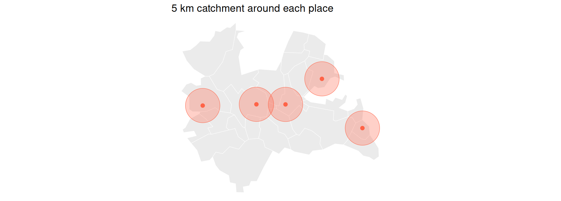
Example: Which Municipalities Border the City?
st_touches()finds polygons that share a border with the city of Utrecht:
neighbours <- st_touches(utrecht_city, utrecht, sparse = FALSE)

ggplot() +
  geom_sf(data = utrecht, fill = "grey92", colour = "white") +
  geom_sf(data = utrecht[as.vector(neighbours), ], fill = "tomato") +
  geom_sf(data = utrecht_city, fill = "steelblue") +
  theme_void() +
  labs(title = "Utrecht city (blue) and its neighbours (red)")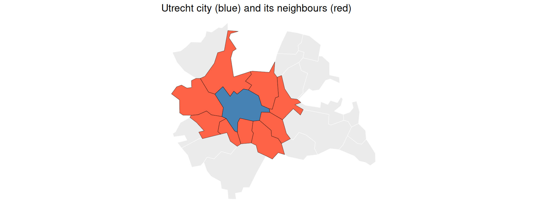
Understanding Bands
- A band is one “layer” of light the satellite sensor records.
- Just as your phone camera has separate sensors for red, green, and blue to build a colour photo, a satellite captures several bands.
- These include light our eyes cannot see, such as infrared, which is useful for measuring vegetation.
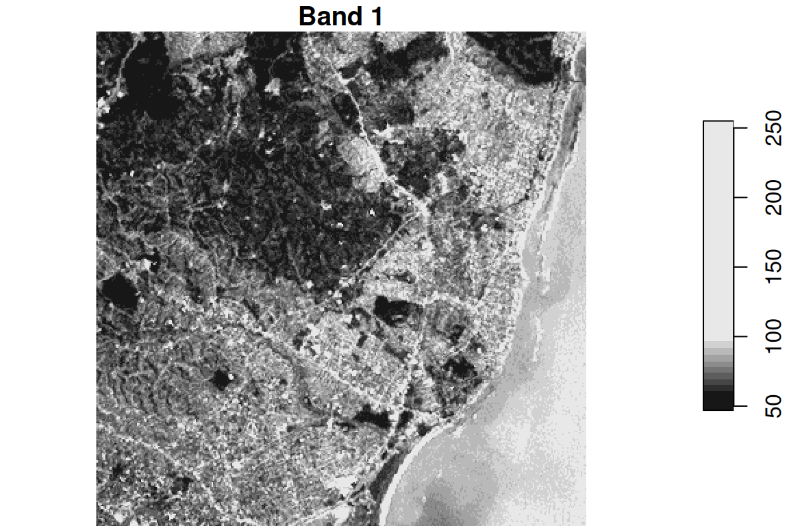
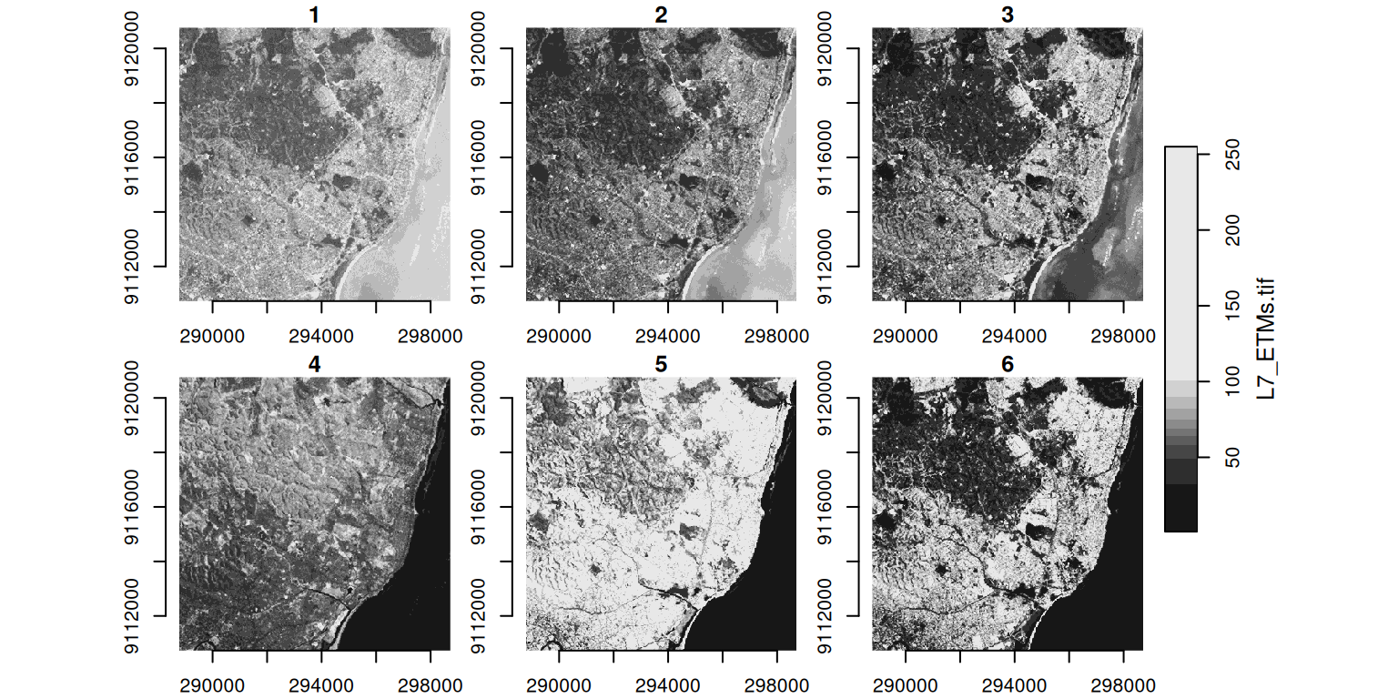
Plotting All Bands
- By default,
plot()shows every band side by side:
Subsetting and Cropping
- You can slice a raster by index (like an array) or crop it to a spatial shape:
   x    y band
 100  100    3
# By shape: keep only what falls inside a circle.
# The point c(293750, 9115745) sits inside the scene, in the image's own CRS.
circle <- st_buffer(st_point(c(293750, 9115745)), 400) |>
st_sfc(crs = st_crs(landsat))
landsat_crop <- landsat[circle]
plot(landsat_crop[ , , , 1], main = "Cropped to a 400 m circle (band 1)")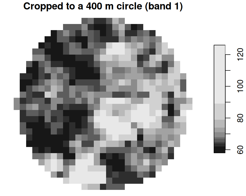
Example: Precipitation per Municipality
Example: Aggregating a Raster over Polygons
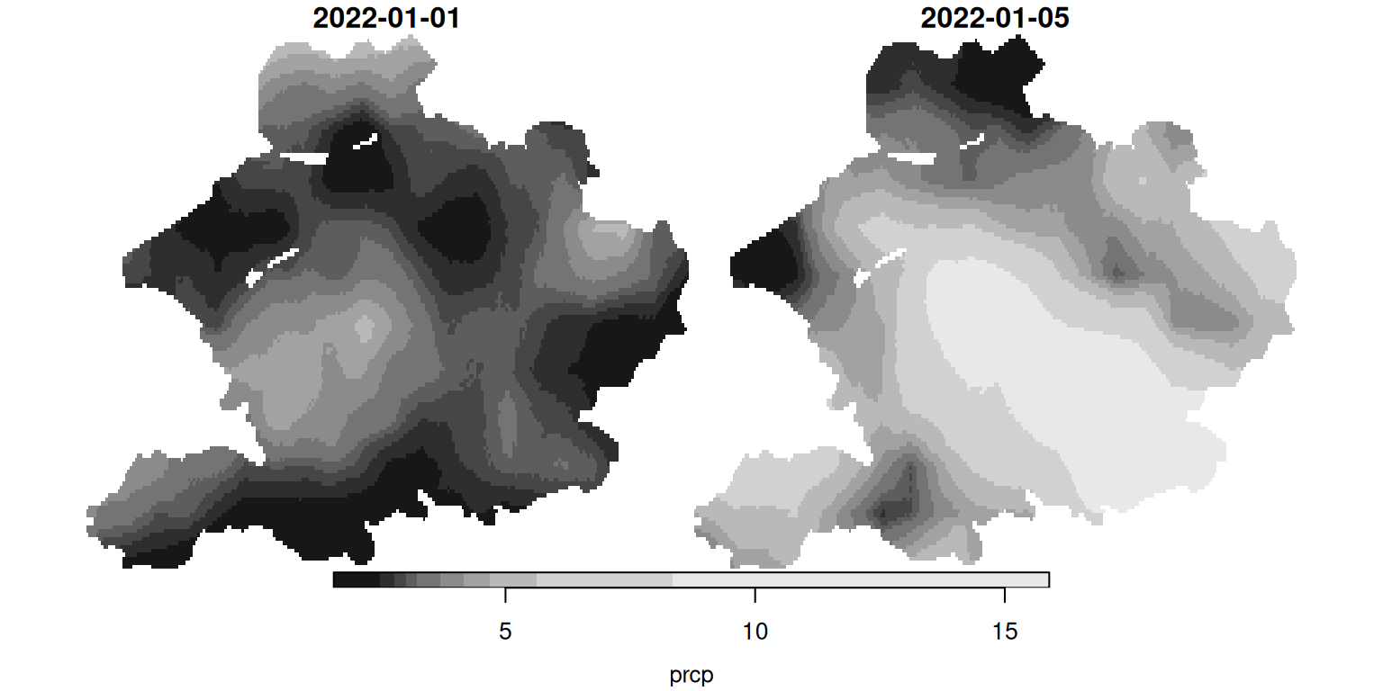
We pull daily precipitation over part of the Netherlands from easyclimate, then average it to municipalities.
Get the raster of daily precipitation:
stars object with 3 dimensions and 1 attribute
attribute(s):
      Min. 1st Qu. Median     Mean 3rd Qu.  Max.   NAs
prcp  1.56     2.9    3.7 4.530697    5.06 15.89 27886
dimension(s):
     from  to offset     delta refsys                 values x/y
x       1 249      5  0.008333 WGS 84                   NULL [x]
y       1 135  52.86 -0.008333 WGS 84                   NULL [y]
band    1   2     NA        NA     NA 2022-01-01, 2022-01-05
The five days, side by side:
Now aggregate to municipalities. Averaging the cells inside each polygon only summarizes values; it never measures a distance or area, so we do not need a metre-based CRS here, and we can keep everything in lon/lat to match the raster.
gemeenten16 <- cbs_get_sf("gemeente", 2016) |>
  st_transform(4326)

# index the time dimension by POSITION (the 1st day) — robust to how the
# date labels are stored, unlike slicing by a "2022-01-01" character label
avg_precip <- aggregate(precip[ , , , 1], gemeenten16, mean)

# aggregate() keeps the rows in the same order as the `by` polygons,
# so we can drop the number straight back onto the vector layer
gemeenten16$prcp <- avg_precip$prcp
We now have one number per municipality, derived from the raster, which we can map like any other attribute:
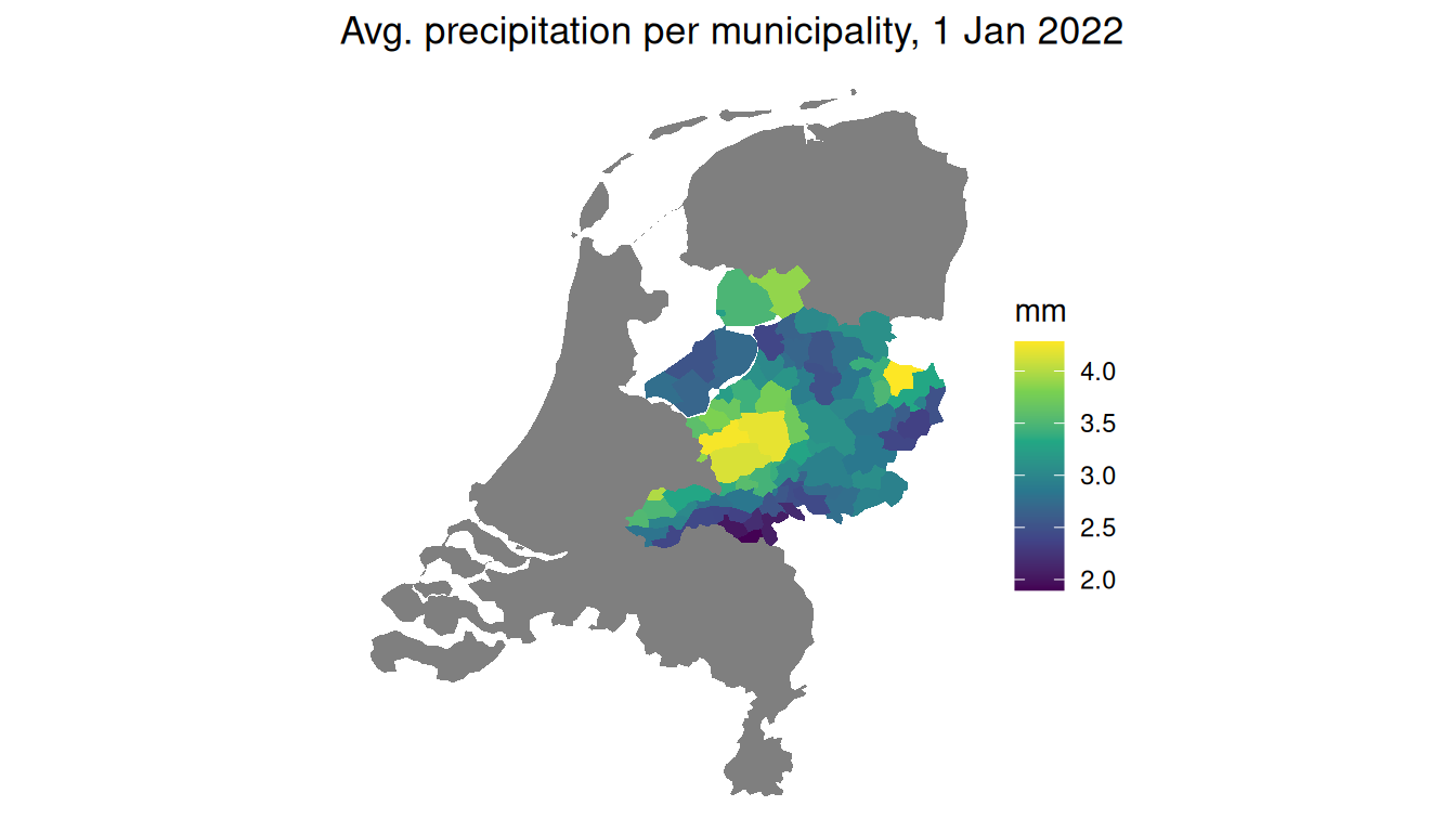
A raster, summarized into a vector map: the workflow you will reach for again and again.